System Gain Calibration
Gain Control "Knobs"
Non-solar radio interferometers can make the assumption that the system noise is dominated by the relatively uniform sky, but this is not at all valid for the Sun--the Sun dominates the system noise, and can be highly variable, especially during flares and other radio outbursts. This is a main reason why it is necessary to design solar-dedicated instruments for observing the Sun. In order to cope with the high and variable noise from the Sun, EOVSA is equipped with a series of attenuators, two RF attenuators in the frontend, and an IF attenuator in the analog downconverter. In addition, it is possible to change the gain via parameters (ADC Attenuation, FFT Shift, and Equalizer Coefficients) in the digital correlator. The table above lists the various gain control points, their purpose, and other relevant information.
Calibrating Front End Power Detectors
There are power detectors in each of the two channels in each front end, just before the optical link, which measure a voltage proportional to the RF power level (integrated over the full 2.5-18 GHz range). To convert these voltages to power measurements, in dBm (decibel-milliwatts), the input of each front end is terminated with a room temperature 50-ohm load, and the output just before the optical link is connected to the E4418B power meter. There is a LabVIEW vi called "E4418B Measurement.vi," to be run on the Win1 computer, that steps the attenuation and performs the measurements both with and without the ND turned on, to range over a wide range of voltages and powers. The vi then writes the result into two text files named, for example,
Antenna 8 HPOL 412016 193307UT.txt
Antenna 8 VPOL 412016 193307UT.txt
There are many more measurements in the text files than needed, and there is no close synchronization between the switched state of the attenuators and the measurement, so one must then edit the file to remove all measurements except one for a given state. Here is an example of an edited file:
HPOWER ND HATTN1 HATTN2 HVOLT VATTN1 VATTN2 VVOLT
10.629 1.000 0.000 0.000 2.280 0.000 0.000 3.406
9.774 1.000 1.000 0.000 1.917 1.000 0.000 2.981
8.982 1.000 2.000 0.000 1.624 2.000 0.000 2.620
7.063 1.000 4.000 0.000 1.086 4.000 0.000 1.880
3.231 1.000 8.000 0.000 0.576 8.000 0.000 0.879
-4.953 1.000 16.000 0.000 0.173 16.000 0.000 0.271
9.791 1.000 0.000 1.000 1.924 0.000 1.000 2.998
8.960 1.000 0.000 2.000 1.616 0.000 2.000 2.617
7.044 1.000 0.000 4.000 1.082 0.000 4.000 1.868
3.160 1.000 0.000 8.000 0.571 0.000 8.000 0.876
-5.139 1.000 0.000 16.000 0.168 0.000 16.000 0.266
6.886 0.000 0.000 0.000 1.045 0.000 0.000 1.841
5.813 0.000 1.000 0.000 0.859 1.000 0.000 1.487
4.881 0.000 2.000 0.000 0.737 2.000 0.000 1.223
2.777 0.000 4.000 0.000 0.540 4.000 0.000 0.825
-1.246 0.000 8.000 0.000 0.303 8.000 0.000 0.457
-9.454 0.000 16.000 0.000 0.081 16.000 0.000 0.137
5.837 0.000 0.000 1.000 0.862 0.000 1.000 1.501
4.861 0.000 0.000 2.000 0.735 0.000 2.000 1.221
2.752 0.000 0.000 4.000 0.537 0.000 4.000 0.820
-1.343 0.000 0.000 8.000 0.300 0.000 8.000 0.452
-9.886 0.000 0.000 16.000 0.076 0.000 16.000 0.127
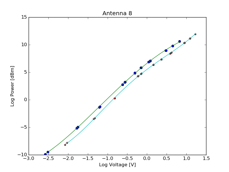
When the edited files are ready, the Python script fem_cal.py is run to create the plot shown in Figure 1 for antenna 8, which includes the measured points and a 4th-degree polynomial fits. The parameters of the fit are printed to the terminal, which for the example in Figure 1 are:
HPOL.c0 =  6.6138626
HPOL.c1 =  5.6355898
HPOL.c2 = -1.0031312
HPOL.c3 = -0.1882171
HPOL.c4 =  0.0348016
VPOL.c0 =  5.5092565
VPOL.c1 =  5.4037776
VPOL.c2 = -0.9535324
VPOL.c3 =  0.3611041
VPOL.c4 =  0.2671788
These lines are then entered into the corresponding crio.ini file, which is located in the crio's /ni-rt/startup folder. The new values will take effect on the next reboot of the crio, or in response to a sync command.
Calibrating the FEM Attenuation Settings
The purpose of the frontend attenuators is to set the optimum base power level for the optical transmitters on the blank sky. FEM stands for Front End Module. The base power level is then maintained automatically by the system when pointing at the Sun or other strong power source (e.g. a satellite) by means of the automatic gain control system (invoked by issuing the AGC command to set the AGC operating parameters, and issuing FEMAUTO-ON to turn it on). To set the attenuations to an appropriate level requires the following calibration procedure.
The calibration of the FEM attenuation settings is very straight-forward. Because the voltage detectors are calibrated to provide power levels, all that is necessary is to read the current power level and attenuation settings from the 1-s stateframe monitor system and determine what attenuation is needed to achieve the desired, fixed power level. The default desired power level is 3 dBm, so if the current power level for an antenna/polarization channel is, say, 5 dBm, one would insert an additional 2 dB of attenuation on that channel to bring the level to 3 dBm. The commands to set the frontend attenuation are HATTN a1 a2 <ant> and VATTN a1 a2 <ant>, where a1 is the setting for the first attenuator, in dB, and a2 is the setting for the second attenuator. The <ant> string, of the standard form (e.g. ant1, or ant1-5) specifies which antenna(s) to apply the settings to. To calibrate the settings, the current power levels and attenuation levels are simply read from the 1-s stateframe monitor system, and any power-level differences from the target 3 dBm are minimized by issuing HATTN and VATTN commands to increase or decrease the current attenuation settings. This can be done from the schedule by means of the $FEM-INIT command, which spawns a process to run the set_fem_attn() routine in the adc_cal2.py module, or the set_fem_attn() routine can be run manually from ipython.
There are some rules and exceptions:
- The power-level measurement is to be made on blank sky (i.e. NOT pointing at the Sun or other strong source such as a satellite).
- The FEMAUTO-OFF setting should be issued (i.e. no automatic gain control), and FEMATTN 0 set (no additional attenuation in the front end), prior to $FEM-INIT. Issuing the $FEM-INIT does not insure the above conditions--these have to be done manually before issuing that command.
- The $FEM-INIT only adjusts ant1-13, because the ant14 power level is allowed to be higher (front end attenuations should always be zero for calibrators, although some attenuation is needed on satellites).
- The calibration settings are remembered by the crio in each antenna by the simple means of writing any HATTN or VATTN settings into the crio.ini initialization file on the crio. Therefore, such settings DO survive a reboot of the crio.
- Note that any inadvertent issuing of an HATTN or VATTN command by hand will overwrite the calibration, and necessitate rerunning the $FEM-INIT command. To avoid this, use the FEMAUTO-OFF and FEMATTN commands instead, to temporarily set an attenuation.
- A few antennas (e.g. the "prototype" frontends on Ant 1, 8 and 11) may not be able to reach 3 dBm power level, even with 0 attenuation. That is not a problem, since the remainder of the signal chain is adjusted to compensate.
Calibrating the DCM Attenuation Settings
SUBARRAY1 ant1-14
DCMAUTO-OFF
FSEQ-FILE solar.fsq
FSEQ-ON
$SCAN-STOP
$CAPTURE-1S dcm
to capture the data for the calibration, then analyze it in ipython (on pipeline, say)
import roachcalExamine the table. Recently, band 1 has had bad attenuations due to RFI, so it underflows on the Sun. If sotbl = roachcal.DCM_calnew('/dppdata1/PRT/PRT<yyyymmddhhmmss>dcm.dat',\ dcmattn=10, missing='ant15')
tbl
tbl = roachcal.override(tbl, bandlist=[1], t=Time('2020-05-08'))
where the t argument gives the date whose SQL table is the source of the override information. If not provided, or None, the SQL table for the current date is used. It is useful to compare the new table with an existing table to check for errors/glitches. To do this, roachcal.compare_tbl(tbl, t=Time('2020-05-08'))
will print a table of attenuation differences. Normally such differences should be small, so large, unexplained differences should be investigated. When satisfied with the table, write a new record to the SQL database. import cal_header cal_header.dcm_master_table2sql(tbl)
The purpose of the DCM attenuator calibration is to ensure optimal ADC (analog to digital converter) levels in the ROACH boards. DCM stands for Down Converter Module. The ADCs take the noise-like variable voltage from the DCMs and convert it to 8-bit digital numbers ranging from -128 to 127. For optimum performance, the ADC level should be as high as possible without clipping. The correlator sends out P (power) packets whose header gives the integrated power for each accumulation. It is useful to record here the relationship between those power levels in the header and the ADC digital numbers. Basically, the time-domain ADC digital values are normalized to +/- 1, squared, and summed over values, then divided by . By trial and error, I find that the correlator reports overflows if the power values exceed 2500, while a more-or-less optimum power level is 1600. Working backward, a power-level can be converted to the typical ADC value by , so for the 200 MHz correlator, where the accumulation length is , this is . The above P values give and , for 2500 and 1600, respectively. This agrees quite well with my experimental results, since for is 114, close to the maximum value of 128.
Unlike the FEM attenuation, which affects the entire RF band, the DCM attenuation is frequency dependent, because it is inserted into the IF signal path after tuning to a specific band. That brings up two complications: (1) a separate DCM attenuation setting is needed for each of the 34 possible IF bands, and (2) the DCM attenuation has to be changed on a 20 ms timescale (50 times/s), in unison with the rapidly switching frequency sequence. Each 20-ms period is called a "slot."
In order to accomplish this feat, whenever the frequency sequence (fsq file) is changed, a new set of attenuations matching that sequence has to be uploaded to the DCMs. This starts with a "master" table of 30 IF channels (2 each for 15 antennas, although Ant 15 is no longer part of the system) for 52 bands. The purpose of the DCM attenuation calibration is to determine these optimal attenuation numbers. Once the master table is defined, the system creates the DCM attenuation table on the fly at the start of each scan, according to the chosen frequency sequence for that scan. The DCM master table size, then, is 30 x 52, from which the DCM table of size 30 x 50 is created at the start of a scan, for the 30 IF channels and 50 "slots." This 30 x 50 DCM table (called dcm.txt) is sent to the ACC (FTP'd to the /parm folder and then commanded to be read by the DCMTABLE command) at the start of each scan. The ACC subsequently uploads the information once to all of the DCMs on the relatively slow RS-485 serial connection. Further modifications to the DCM attenuation are possible on a 1-s cadence, issued by the DPP.
The procedure for creating the master calibration table (the 30 x 52 table) is to first ensure that the dishes are off the Sun, the FEM attenuations are properly set via the $FEM-INIT schedule command, and a suitable frequency sequence is running that samples all 52 bands. Currently, the solar.fsq sequence is defined for this purpose. Stop the DCM attenuation switch by issuing the DCMAUTO-OFF command. This will set the DCM attenuations on Ants 1-13 to a fixed 10 dB. With the dppxmp program idle (i.e. with $SCAN-STOP in effect), perform a 1-s packet capture on the DPP (can be done with the $CAPTURE-1S schedule command, or just type capture in a dpp terminal window). A new capture file named PRTyyyymmddhhmmss.dat will appear in the /data1/PRT folder on the DPP (or /dppdata1/PRT folder on pipeline or tawa). To analyze the packet capture file and update the SQL database, in ipython on the dpp, pipeline, or tawa, issue the following commands:
import roachcal tbl = roachcal.DCM_calnew(<filename>, dcmattn=10, missing='ant15') tbl
Note that this is an update from the old 34-band analysis, which was done using the roachcal.DCM_cal() routine. This old routine is kept unchanged in case we ever need to go back to the previous 34-band setup (not anticipated!). The above commands will print the 30 x 52 master table to the terminal window. Examine the table for any errors. In particular, here, it is important to list any non-working antennas (ant15 is always non-working) in the "missing" parameter, so that the routine knows not to update the attenuations for those. A common error is to not specify a non-working antenna, which may show up as no signal, and hence the analysis will result in setting those DCM attenuations to zero (in an attempt to increase the signal level). When the antenna comes back online, the DCM table will indicate zero attenuation, and now the ADC level will be very large and potentially damage the ADC! Once you are happy with the contents of the table, issue these commands to write the result to the SQL database:
import cal_header
cal_header.dcm_master_table2sql(tbl)
Note: cal_header.dcm_master_table2sql() also has a tbl=tbl parameter, but this expects an array of numbers, not an ASCII table of the type returned by roachcal.DCM_cal(), so calling it as tbl=tbl will fail.
New Calibration Procedure
Since late 2021, a new procedure has been established to determine, create, and send the DCM Master Table to the SQL database. The procedure uses the always running new procedures in adc_plot.py. In the past, the DCM attenuations were based on the information in the correlator packets (using packet capture). Now we are measuring the ADC values directly once per minute and writing them to a file on the DPP. Therefore, a more direct means of determining the DCM levels is based on setting up the analog system for measuring fixed ADC levels, and then using those measurements to create the table. The setup is similar to the above, i.e.,
stow
$scan-stop
femauto-off
femattn 0
$fem-init
dcmauto-off
fseq-off
fseq-init
fseq-file solar.fsq
fseq-on
Then let the system remain in this mode for 10 minutes to enable 10 measurements of the ADC levels to be written into the dpp:/tmp/ADCplot<yyyymmdd>_<hhmm>.npy file. In ipython, you can watch the levels by
import adc_plot as ap
from util import Time
ap.adc_plot('/tmp/ADCplot<yyyymmdd>_<hhmm>.npy')
which will open a multi-panel plot and show the levels once per minute as they are taken. When 10 minutes of good measurements have been acquired, close the plot, which will (eventually) stop the adc_plot() routine. Or you can just ctrl-C out of it. When the ipython prompt is again ready, issue a command like (the example below is for a particular date and time):
ap.adc2master_table('/tmp/ADCplot20211212_1100.npy',Time('2021-12-12 15:50'), attnval=14)
and you will see the table printed to the screen along with a question:
Do you want to write this to the SQL database DCM master table? [y/n]?
Entering y will send the table to SQL.
To test the new gain settings, send the sequence of commands
fseq-off
fseq-file solar.fsq
fseq-on
dcmauto-on
and restart the adc_plot to see the new levels. After a minute or two they should appear flat near the optimum level on all antennas.
Calibrating the Correlator EQ coefficients
The purpose of the equalizer coefficients is to set the power level in the correlator for optimum 4-bit sampling. The way to verify a correct setting is to compare the high-precision accumulated power with the accumulated 4-bit autocorrelation power. When the settings are correct, these two should be identical. Note that the procedure described here is under development and will likely change in some details. --Dgary (talk) 13:06, 22 April 2017 (UTC)
When the FEM and DCM attenuations are properly set, the power level measured in the correlator should be roughly constant, independent of band, as the system rapidly tunes during the 1-s frequency sequence. However, this is only the integrated power level over the IF band. The power level over the 4096 subchannels within a band can vary, mainly due to the bandpass shape. To keep everything optimum for good linearity of the correlated data, the autocorrelation power on a 4096 subchannel basis should match the power. Therefore, the EQ coefficients have sufficient resolution (128 separate coefficients over the 4096 subchannels, each adjusting 32 contiguous subchannels) to flatten the bandpass, with a separate array for each of the 50 slots of a 1 s sequence. So far, we have only set the EQ coefficients to a constant, with the same value applied to all antennas, all bands, and all 128 values across each band.
The basic procedure envisioned for this calibration is to set an all-band observing sequence (e.g. gaincal.fsq) and then packet-capture data over a range of constant EQ coefficient settings, then analyze the packet-capture files to determine what setting results in the best agreement between power and autocorrelation for each antenna, polarization, band, and 32-subchannel subband. Unfortunately, this has to be done with packet-capture data because we need the 4096-subband resolution, and although it takes only 1 s to capture a file for one EQ setting, it takes about 1 min to read such a file (1 GB) and analyze it. One can imagine that, once things are set close to optimum, a set of captures over 4-5 EQ settings would be sufficient, and so the entire procedure could be done in 5 minutes. It remains to be seen how variable this is over time, and whether the settings are substantially different off and on the Sun.
Setting ADC Level (tests)
We have devised a way to conveniently measure the ADC levels using the snapblocks in the correlator. The 8-bit ADCs directly measure the (digitized) voltage of the IF band, and can measure values ranging from -128 to +127. For a noise-like (Gaussian-distributed) signal, the optimum setting would be one that very seldom (or never) exceeds these limits, but comes as close as possible. Each time-domain voltage sample for a 4096-point spectrum consists of 8192 data points, so if we set 4 = 128, we expect 0.000133*8192 = 1.1 of the values to overrun. Thus, we want to set the signal such that the standard deviation is 1 = 32 in ADC units.
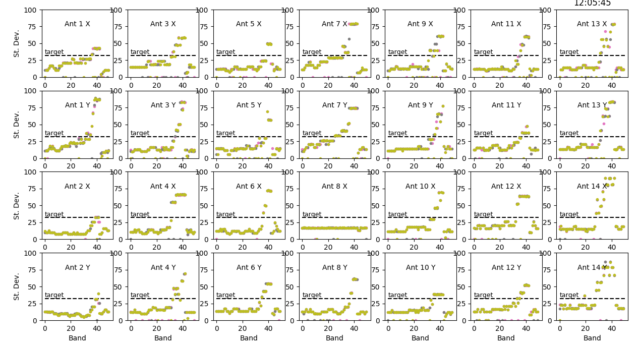
Because we are switching bands every 20 ms, it is a bit tricky to ensure that we are grabbing ADC snaps on each band (it is a matter of controlling the timing of the snap), but some code has been written that does this relatively successfully for both IFs on each antenna at each of the 50 slots. When we run the solar.fsq frequency sequence, which measures a different band in each slot, we therefore can obtain all relevant ADC levels about once per minute. So long as we ensure that the input signal is relatively stable, we can get a nice, repeatable measure of the ADC levels. By holding both the front end (FEM) and back end (DCM) attenuations fixed, we obtain something like Figure A.
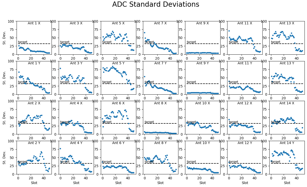
It is clear that the ADC levels vary quite a bit with antenna, IF, and band, but for optimal performance we want to manipulate the levels so that all of the points are as close as possible to the target level of 32 (black dashed line in each panel) without being above it. In fact, we can easily use the measured ADC levels to estimate the required DCM attenuation needed to correct them to match the target. Given the data at one time data[1], the required attenuation for an initial DCMATTN setting of 10 will be attn10 = log10(((data[1]/32.)**2))*10. + 10. When the initial DCMATTN setting is 14, the corresponding attn will be attn14 = log10(((data[1]/32.)**2))*10. + 14. Figure B shows the DCM attenuation values for these two cases for the same data as in Figure A. There are two sets of points shown, blue ones for attn10 and orange for attn14. It is clear that they agree very well such that the blue points are hardly visible.
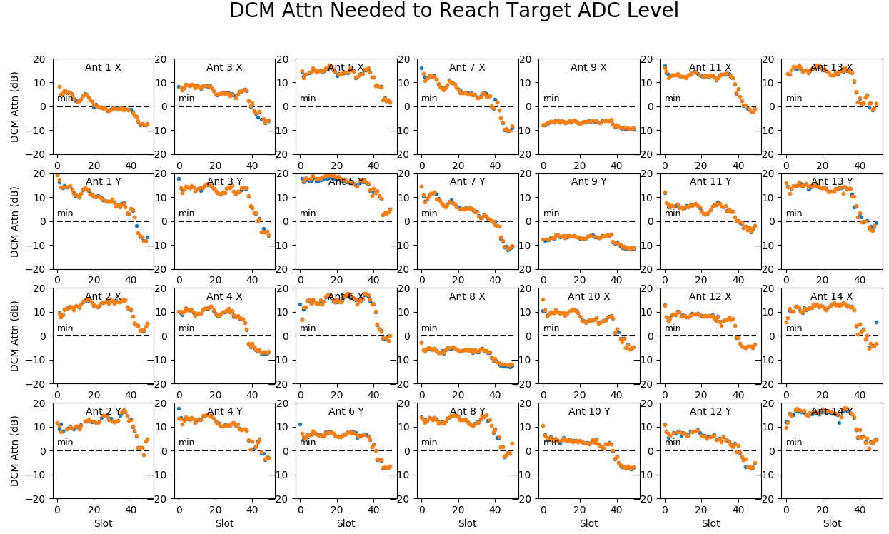
Of course, points in Figure B that are below 0 dB (the dashed line marked "min") cannot be fully corrected since we cannot set the DCM attenuation to less than zero! Antenna 9 does not count here, because that antenna was non-functional when the data were taken. However, the X channel of Antenna 8 is entirely below zero, as are the high-frequency points in many of the IFs. Those will have DCM attn set to zero, but will remain below the target ADC value.
Discovery and Solution of a Problem
After being able to monitor and predict the ADC levels as above, the DCM attenuations were set appropriately to leveling the ADC standard deviations at all bands, but it immediately became apparent the the corrections did not work as expected! It is clear that there is some sort of bug in the DCM attenuation states. This looked very serious, since the results were apparently scrambled in ways that were not obvious. However, today I (--Dgary (talk) 14:10, 9 May 2021 (UTC)) devised a means to measure the attenuation state of the DCMs directly, and as a result I verified that the error is only one of timing. It appears that the attenuation states are being correctly applied, but not at the right time.
What I did for the test was to allow the DCM attenuations to cycle according to the solar.fsq sequence, and then set the fseq file to a fixed frequency (band10.fsq). In that situation, the IF level in was constant, so any variations in the ADC levels had to be due solely to the DCM attenuation switching. Running that test resulted in Figure C. Taking the first measurement of each antenna/channel as a reference, I was then able to determine the relative attenuation in dB for every band (slot). To my satisfaction, the values perfectly corresponded to multiples of 2dB, as expected.
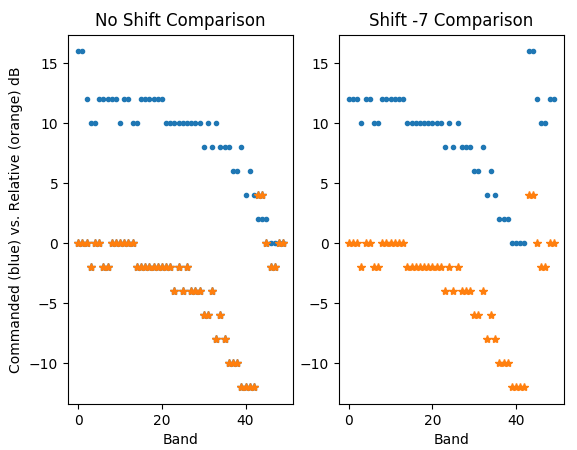
A relatively few python commands, as in the following script, suffice to show the situation, resulting in Figure D. As Figure D (right panel) shows, the commanded attenuations are happening, but 140 ms late (a shift of 7 20-ms slots). This is a disaster as far as correcting for power levels, because now the high attenuations needed at low frequencies are actually being applied to the high frequencies!
# Read stdout file
import struct
fh = open('/tmp/stdout20210509_1156.dat','rb')
buf = fh.read()
fh.close()
data = array(struct.unpack('14000d',buf))
data.shape = (10,28,50)
slot = arange(50)
data[where(data < 0.00001)] = nan
# Find median of repeated values for samples 4-10
blah = nanmedian(data[4:],0)
# Calculate attenuation relative to first measurement
blah0 = blah[:,0].repeat(50).reshape(28,50)
rattn = -np.round(log10(blah/blah0)*10*2)
# Read current table from SQL
import cal_header
import stateframe
xml, buf = cal_header.read_cal(2)
cur_table = stateframe.extract(buf,xml['Attenuation'])
# Indexes that skip unused bands 2 and 3 of the 52 possible
good = array([ 0,  1,  4,  5,  6,  7,  8,  9, 10, 11, 12, 13, 14, 15, 16, 17, 18,
       19, 20, 21, 22, 23, 24, 25, 26, 27, 28, 29, 30, 31, 32, 33, 34, 35,
       36, 37, 38, 39, 40, 41, 42, 43, 44, 45, 46, 47, 48, 49, 50, 51])
# Plot a comparison for one channel (this is random channel k=23, which is Ant12 Y)
f, ax = subplots(1,2)
ant=12
pol=2
k = (ant-1)*2 + pol-1
ax[0].plot(roll(cur_table[good,k],0),'.',color='C0')
ax[0].plot(rattn[k],'*',color='C1')
ax[1].plot(roll(cur_table[good,k],-7),'.',color='C0')
ax[1].plot(rattn[k],'*',color='C1')
ax[0].set_title('No Shift Comparison')
ax[1].set_title('Shift -7 Comparison')
ax[0].set_ylabel('Commanded vs. Relative dB')
ax[0].set_ylabel('Commanded (blue) vs. Relative (orange) dB')
ax[0].set_xlabel('Band')
ax[1].set_xlabel('Band')
What is nice, though, is that the 7-slot shift is exactly the same for all channels, which suggests an easy fix, at least for now. I can simply command the attenuation changes early, or in other words shift the DCM.txt list by 7 before I send them to the DCMs. However, I do not know the cause of this shift, so I cannot know if it can change over time, so we will have to monitor the situation. Luckily, the above procedure provides us with an easy way to monitor it. Note that when this shift is done, it should result in a huge improvement in the data quality, which presumably has been messed up since day 1! It turns out this problem is due to an ACC timing error, which was corrected by rebooting the ACC, so the problem only started in late Jan (and got progressively worse).
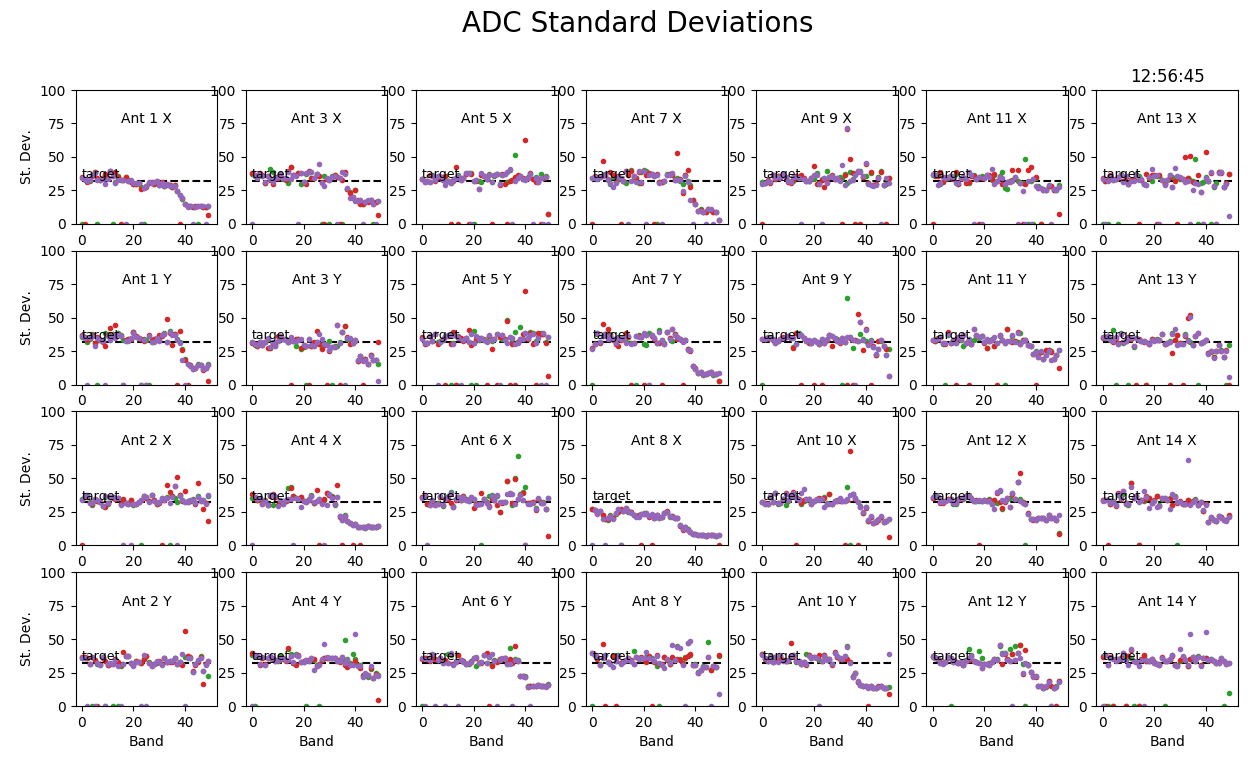
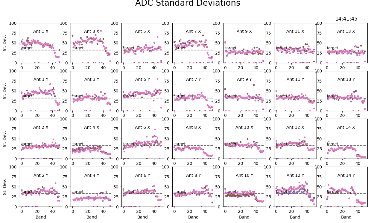
I was able to easily make the adjustment, so now the data look good. See Figures E and F. It turns out that this problem was due to an ACC timing error, which was fixed by rebooting the ACC, so the "adjustment" has now been removed again.
Correlator Non-Linearity
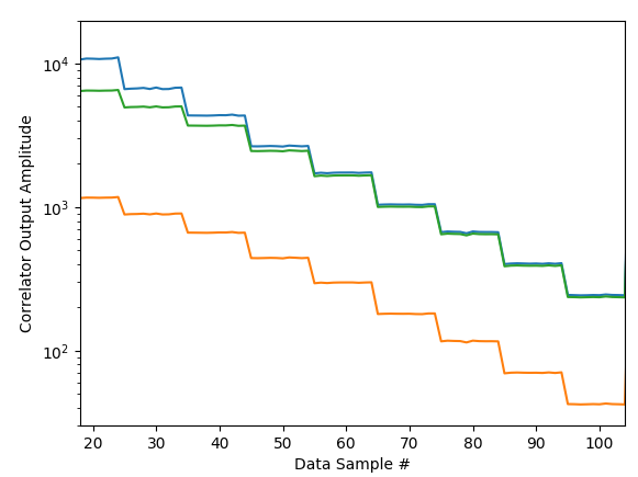
In January 2021 it came to our attention that although the total power calibration provides good numbers for the attenuator settings in the system that corrects the total power well, those same attenuator settings when applied to auto-correlation often give poor results. Those same poor results also affect the cross-correlation amplitudes! To understand the problem, the GAINCALTEST observations were analyzed not only for total power, but also auto-correlation, which clearly revealed the source of the problem. As shown in Figure 2, the auto-correlation. The result of this is that when the power level is high and an attenuation step is introduced, the auto-correlation drop in amplitude is far less than in total power such that correcting such a step based on the total power step greatly overestimates the auto-correlation power. As noted, this same adjustment is applied also to the cross-correlation.
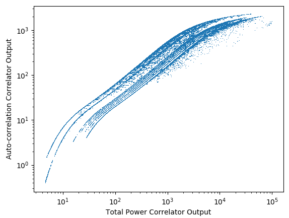
In order to further understand this compression (saturation), the auto-correlation amplitude is plotted against total power amplitude in Figure 3. One can see several curious behaviors in this plot. For one thing, the points seem to organize themselves in discrete curves (aside from some errant points scattered about). Further investigation showed that these curves are organized according to band, with band 1 (lowest frequency) being the left-most curve and successively higher bands shifted discretely to the right. Not apparent in the plot is that the right-most curve contains vastly more points than the others because it is the data for bands 10-52, all landing on top of each other.
The shifts of the other curves is simply due to the differing bandwidths of individual science channels in those lower bands. At first this seemed like it might be reasonable, but as I think about it I think this is very unwanted behavior! It must be that the dppxmp software is doing some correction to either auto-correlation or total power but not the other! This is probably largely taken out by the scheme we follow for total power calibration, but it is not correct. I'll investigate this and probably make a change to eliminate this effect for future data.
What is truly remarkable is that this universal curve, shifted only due to differing bandwidth, is exactly followed in all GAINCALTEST measurements, day after day, with each measurement following precisely the same curve. This shows that it is a purely digital effect in the correlator having to do with the finite range of the 4-bit down-sampling of the total power to create the auto-correlation. There is a correlator parameter that can be adjusted, but clearly the range of total power exceeds the linear range of the 4-bit sampling. Still--it is worth investigating.
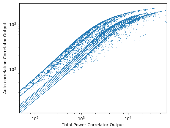
Our immediate interest is in finding a correction to apply to the auto-correlation to correct for this easily predicable effect, and especially at the higher end since the higher power levels is where the correlator is mainly operating. Only 10% of points have auto-correlation amplitude less than 20. Figure 4 shows a zoomed version of Figure 3, concentrating on the higher power end of the range. In this log-log plot, the curve has a smooth behavior reminiscent of an error function, so a trial fit of a function of this form was attempted with excellent results. Using = total power level and = auto-correlation level, the function
where and fits the function extremely well. Once the total power is adjusted for bandwidth, a universal fit with parameters and fits very precisely for all antennas, polarizations, frequencies and times. Conversely, we can modify parameter for bandwidth by where is the number of science channels in a band. Figure 5 shows some fits to actual data using this function with these parameters.
Using this function with these parameters, it should be a simple matter to simply use the measured total power value to calculate a correction factor to apply to the auto- and cross-correlation to correct for the saturation. This will be done in the udb_corr() routine of pipeline.py. It has to be applied to the initial data from read_idb() before any corrections.
Because the function is most linear at its midpoint, given by the zero of the function, we will take the value at as the "correct" value and seek to find the line with unit slope that goes through that point, which is the line . Thus, the correction factor to apply to to make it become is
and the final correction to the auto-correlation is . This same correction is needed for cross-correlation, i.e. for cross-correlation on baseline , the corrected value is .
Note: I tried applying this to correct some GAINCALTEST data, and it works very well for power levels that are sufficiently high. However, it fails badly for low power levels. It is easy to see why by looking at Figure 3, where the curve turns downward at low auto-correlation values. The erf correction actually turns upward there, so it is a bad approximation at low auto-correlation levels. It is better if I only correct data with auto-correlation > 50 or so. I will set for auto-correlation levels less than 50. Spot checks of this show that the result looks great.
This correction needs to be done prior to any other manipulations of the data, hence it should be applied for all calibrations (SKYCAL, GAINCALTEST, SOLPNTANAL, etc.). Making this change means that such calibrations need to be redone before they can be used. I will look for a software solution that is as efficient as possible.
More on the correlator saturation
After making the adjustments to the ADC levels in the previous section (in May 2021) I find that the saturation is now much worse. This is to be expected since the ADC levels are now generally higher and so more saturated at the correlation stage. Today I --Dgary (talk) 14:32, 16 May 2021 (UTC) changed the equalizer coefficients from 8.0 to 2.0 for all IFs after doing some GAINCAL tests. This results in much less saturation, but has also changed the behavior so that the above expression no longer works. Therefore, a new expression will be needed. I will work on that and give it here when it is available. Meanwhile, the desat correction will not be the right one for any data taken until a new expression is determined, so all pipeline analysis will have to be redone from today until this is corrected.
Within a day or two, a new correction was determined and is now being applied for data since 16 May 2021. In this case, a single functional form did not fit the data as well, but a compromise was made to fit amplitudes below 300 with one function and amplitudes above 300 with another. The two functions have the same form as above, and are applied in the same manner:
with




![{\displaystyle f(x)=a\ {\rm {erf}}{\Bigl [}{\frac {x-c}{b}}{\Bigr ]}+d}](https://wikimedia.org/api/rest_v1/media/math/render/svg/6667a2464fd97b3db5d4758f3129080194a53be8)




![{\displaystyle \eta ={\frac {f^{\prime }(x)}{f(x)}}={\frac {x+d-c}{a\ {\rm {erf}}{\Bigl [}{\frac {x-c}{b}}{\Bigr ]}+d}}}](https://wikimedia.org/api/rest_v1/media/math/render/svg/85b976dbdf56a0c30e4075f1fb50218968efd81d)


![{\displaystyle \eta ={\frac {f^{\prime }(x)}{f(x)}}={\frac {x+d_{i}-c_{i}}{a_{i}\ {\rm {erf}}{\Bigl [}{\frac {x-c_{i}}{b_{i}}}{\Bigr ]}+d_{i}}}}](https://wikimedia.org/api/rest_v1/media/math/render/svg/f628655f14dbc1d524edd3d4c9ae899311619282)
![{\displaystyle a_{1},b_{1},c_{1},d_{1}=[0.88025122,1.0221639,4.39845723,2.38911615]}](https://wikimedia.org/api/rest_v1/media/math/render/svg/a83263af3f8f66fd42108d10c4de3bffa84f7899)

![{\displaystyle a_{2},b_{2},c_{2},d_{2}=[2.28517281,2.64619331,4.38657476,2.37753165]}](https://wikimedia.org/api/rest_v1/media/math/render/svg/b529eff5eac211dcc65a62a3c2fd00ed3d4d0df8)
