Caius' Notes: Difference between revisions
No edit summary |
No edit summary |
||
| (3 intermediate revisions by the same user not shown) | |||
| Line 31: | Line 31: | ||
To verify the antennas that were working, check the observing log http://ovsa.njit.edu/wiki/index.php/2024_May, | To verify the antennas that were working, check the observing log http://ovsa.njit.edu/wiki/index.php/2024_May, | ||
or consult the TPCAL log file, e.g. more /dppdata1/TPCAL/LOG/TPCyyyymmdd.log | |||
Create the flare directory at /data1/dgary/solar/, e.g: | Create the flare directory at /data1/dgary/solar/, e.g: | ||
| Line 74: | Line 75: | ||
Use the figure above to choose the background interval (bgidx), the maximum intensity and the frequencies. | Use the figure above to choose the background interval (bgidx), the maximum intensity and the frequencies. | ||
The tpk | The tpk (Time of the peak) determines the name of the resulting files (.png and .fits): | ||
<pre style="font-family:courier"> f, ax0, ax1 = fs.make_plot(out,bgidx=[200, | <pre style="font-family:courier"> f, ax0, ax1 = fs.make_plot(out,bgidx=[200,210],vmin=0.1, vmax=110, lcfreqs=[120,190,270,350],ant_str='ant1-6 ant8-9 ant11-13', tpk='2024-05-07 16:30:00') </pre> | ||
[[File:eovsa.spec.flare_id_20240507163000.png|none|thumb|center|500px|]] | [[File:eovsa.spec.flare_id_20240507163000.png|none|thumb|center|500px|]] | ||
| Line 84: | Line 85: | ||
In this example, the output files are eovsa.spec.flare_id_20240507163000.fits and eovsa.spec.flare_id_20240507163000.fits. | In this example, the output files are eovsa.spec.flare_id_20240507163000.fits and eovsa.spec.flare_id_20240507163000.fits. | ||
At the end, copy .fits file to /common/webplots/events/2024: | At the end, copy the .fits file to /common/webplots/events/2024: | ||
<pre style="font-family:courier"> cp eovsa.spec.flare_id_20240507163000.fits /common/webplots/events/2024 </pre> | <pre style="font-family:courier"> cp eovsa.spec.flare_id_20240507163000.fits /common/webplots/events/2024 </pre> | ||
Latest revision as of 17:21, 4 June 2024
EOVSA flare spectrograms
Checking the possible EOVSA
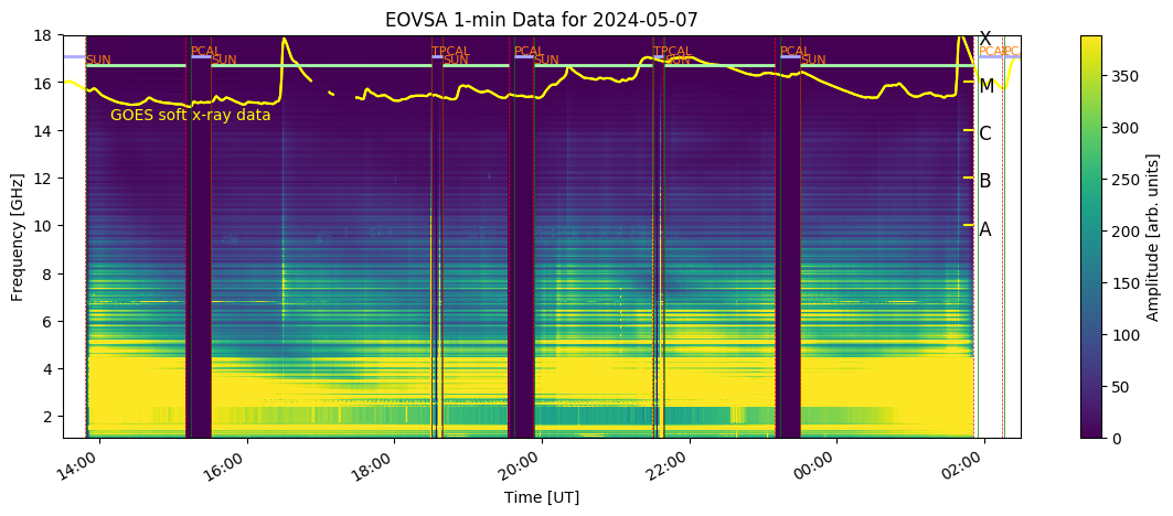
Verify the possible flares on the daily EOVSA Solar Dynamic Spectrogram, for example:
http://ovsa.njit.edu/browser/?suntoday_date=2024-05-07
In this example, we are going to analyze the M8.2 flare that happened after 16:00 UT.
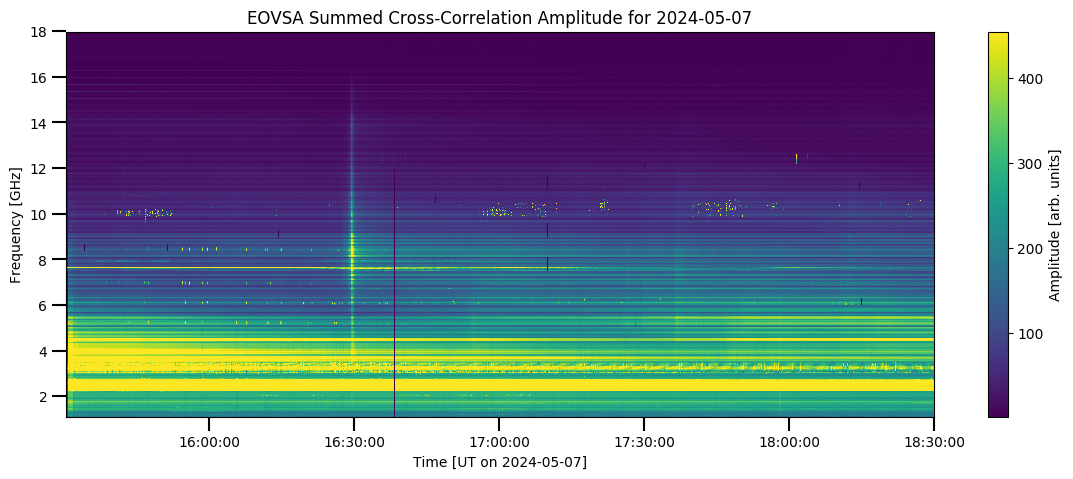
For a better flare time precision, a Dynamic spectrogram with short time range at:
http://ovsa.njit.edu/flaremon/
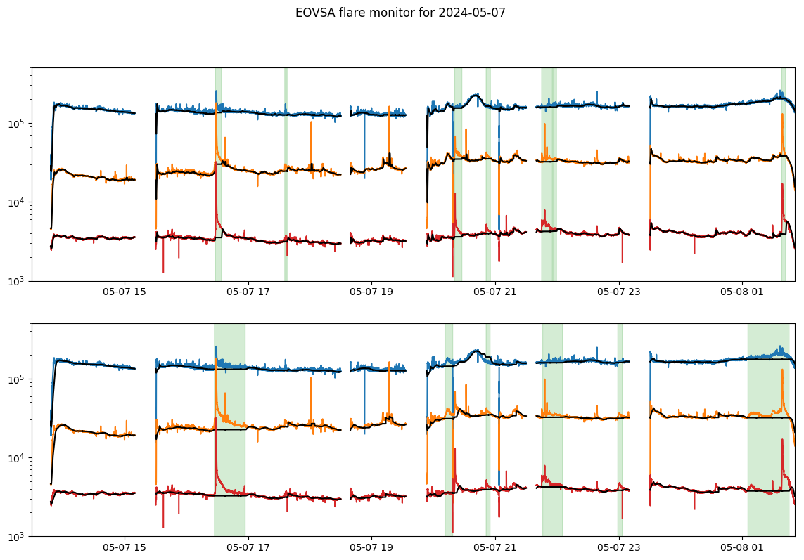
Since 2024-May-05, the Real Time Flare detection figure and its list are also available:
http://ovsa.njit.edu/flaremon/FLM20240507.png http://ovsa.njit.edu/flaremon/flarelist/flarelist_2024-05-07.txt
Using Python 3.8
Login into pipeline machine as user:
ssh -X user@pipeline
To verify the antennas that were working, check the observing log http://ovsa.njit.edu/wiki/index.php/2024_May,
or consult the TPCAL log file, e.g. more /dppdata1/TPCAL/LOG/TPCyyyymmdd.log
Create the flare directory at /data1/dgary/solar/, e.g:
mkdir 20240507_M8flare
cd 20240507_M8flare
Load the Python 3.8 environment:
bash
loadpyenv3.8
ipython --pylab
In Python, enter the following:
from eovsapy import flare_spec as fs
from eovsapy.util import Time
To download the IDB directories form the SQL cloud, enter the flare interval as:
files = fs.calIDB(Time(['2024-05-07 16:20','2024-05-07 16:35']))
If the IDB already exist, they can be read as:
files = ['IDB20240507162024','IDB20240507163024']
When all the antennas were fine, enter the following:
out, spec = fs.inspect(files)
But, if one or more antennas weren't working, enter the list of the good ones as:
out, spec = fs.inspect(files, ant_str='ant1-6 ant8-9 ant11-13')
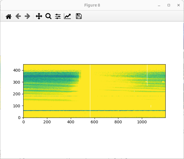
To better see the flare, you can change the spec vmax as:
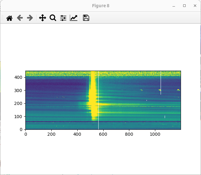
imshow(spec,vmax=30,vmin=-1)
Use the figure above to choose the background interval (bgidx), the maximum intensity and the frequencies. The tpk (Time of the peak) determines the name of the resulting files (.png and .fits):
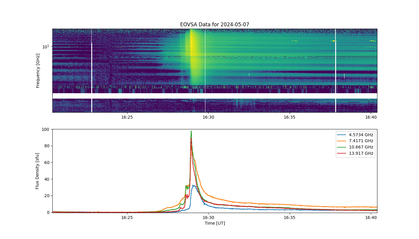
f, ax0, ax1 = fs.make_plot(out,bgidx=[200,210],vmin=0.1, vmax=110, lcfreqs=[120,190,270,350],ant_str='ant1-6 ant8-9 ant11-13', tpk='2024-05-07 16:30:00')
A second background interval can be defined right after the first one, e.g., bg2idx=[1000,1010]
In this example, the output files are eovsa.spec.flare_id_20240507163000.fits and eovsa.spec.flare_id_20240507163000.fits.
At the end, copy the .fits file to /common/webplots/events/2024:
cp eovsa.spec.flare_id_20240507163000.fits /common/webplots/events/2024
and include the flare in the wiki Flare List:
http://ovsa.njit.edu/wiki/index.php/2024
The flare position have been copied from the https://solarmonitor.org/
