Practical Calibration Tutorial

This page is a practical tutorial for calibrating EOVSA data. Note currently the calibration processes can only be done on EOVSA site machines (such as pipeline), as the calibration SQL database is only available there.

Preparation

First, identify whether or not EOVSA had the observation for the time range of the event (e.g., a flare). There are many ways to do this, but a nice way is to use the RHESSI Browser and check "EOVSA Radio Data" on the upper left. Use the time you identified to find the corresponding IDB file(s) under /data1/eovsa/fits/IDB/yyyymmdd/. *Typically*, each IDB data file has a 10-minute duration. Then, on pipeline, it is advised to go to your own directory and work under there. Note, never, NEVER, work directly on the IDB data in the original data directory! Here I use a 10-min duration data on 2017 Aug 21 (which has a C flare) as an example.

Check Status of Calibration Products

Check the calibration status page for status of the calibration products. Navigate to the date of interest and check the numbers under "r" (reference phase), "p" (daily phase calibration), and "tp" (total-power and attenuation calibration). "1" means the respective calibration product already exists. "0" means otherwise.

Reference Calibration and Phase Calibration

If the calibration does not exist for a particular day (i.e., "0"), if you know what you are doing, run the following line on pipeline:

python /common/python/current/calwidget.py &

Follow the prompts in the widget to solve for reference and phase calibration. Flag bad data if necessary, and save the results to the SQL database by clicking on the "Save to SQL" button.

Total-Power and Attenuation Calibration

Checking total-power calibration quality

As introduced in this page, the total-power and absolute flux calibration is done by comparing with RSTN daily radio flux density measurements. It is always a good idea to check the quality of the calibration. To do that, first, start IPython in your working directory. Here I am loading all pylab modules (I know this is not a good way, but simple).

ipython --pylab

Check the quality of the absolute flux (total power) calibration for the particular day

In [1]: from util import Time
In [2]: import daily_xsp
In [3]: daily_xsp.cal_qual(Time('2017-08-21'))

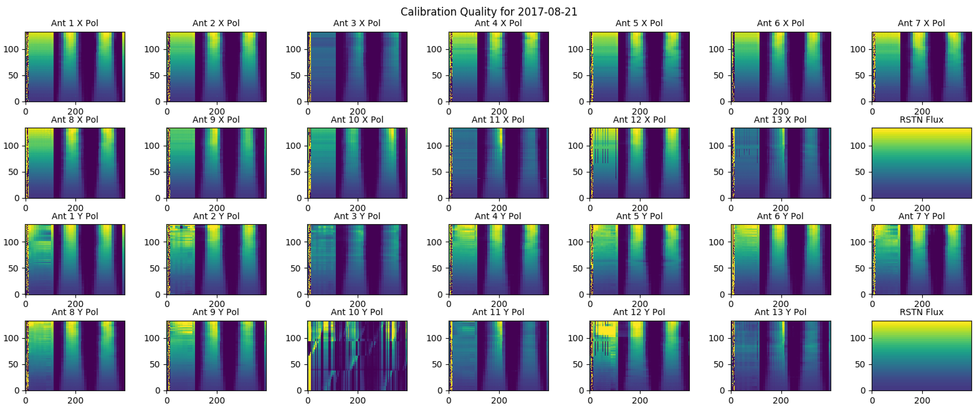
This command will apply attenuation calibration and feed rotation from the database to total-power gain calibration data, and display a figure on the right showing the calibrated total-power spectrum on all antennas and all polarizations. The first scan on the figure is done with the array dwelling on the Sun and stepping through different attenuator levels. The second and third scans are done by moving across the solar disk. A perfect calibration would achieve something similar to the RSTN flux for all antennas and all polarizations. This is not always the case, however. But it helps us to evaluate the quality of the absolution gain calibration.

If the calibration is deemed not satisfactory, one could go back and re-generate the attenuator gain calibration (perhaps it was not generated in the first place). This can be done by running the following command on pipeline (you need to change the date for your desired data)

python /common/python/current/calibration.py '2017-08-21 21:36'

Note the time used here (21:36). Typically, two calibrations are done on 17:30/18:30 and 21:30. Each calibration takes about 5 min. The time selection indicates that we use the second calibration, and make sure that we wait until the second calibration is done.

Apply All Calibrations to Visibility Data

Start CASA in your working directory (e.g., /data1/bchen/). To start CASA, use:

casa

importeovsa

The level 0 visilibity data is in Miriad format (IDB). We should import IDB data into CASA Measurement Set so that we can process the data in CASA. By default, we apply the total power and attenuation calibrations at this stage (via keyword "udb_corr = True"). Multiprocessing can be enabled by setting ncpu = [a number > 1 but < # of available threads].

from astropy.time import Time
import os
trange = Time(['2017-08-21 20:15:00', '2017-08-21 20:25:00'])
#### (Optional) change output path, default current directory "./" #####
outpath = './msdata/'
if not os.path.exists(outpath):
    os.makedirs(outpath)
######################################################
msfiles = importeovsa(idbfiles=trange, ncpu=1[, visprefix=outpath])

calibeovsa

SunCASA task "calibeovsa" applies the reference phase and daily phase calibrations to the visibility data (as a measurement set). After that, the measurement set is calibrated. Calibeovsa also allows to concatenate multiple measurement sets (e.g., several 10-min duration solar files) into a single measurement set.

# This is to set the path/name for the concatenated files
concatvis = os.path.basename(msfiles[0])[:11] + '_concat.ms'
vis = calibeovsa(msfiles, doconcat=True, concatvis=concatvis[, msoutdir=outpath])