Calibrator Survey: Difference between revisions
No edit summary |
(Added Figure 2) |
||
| Line 59: | Line 59: | ||
ax3[j,k].set_ylim(-4,4)</pre> | ax3[j,k].set_ylim(-4,4)</pre> | ||
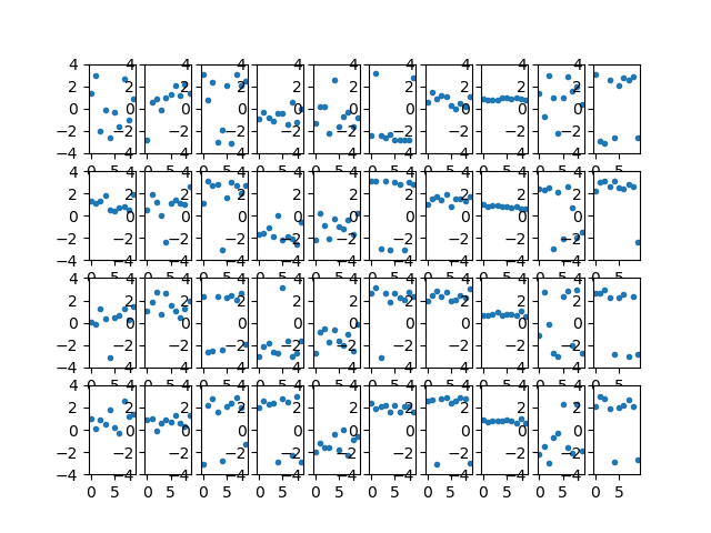
4. If there's nothing going wrong with the observation or its setup, then you should see your phase plots being relatively straight over time, like in Figure 2. If not, there could be something wrong, or you could wait another 10 minutes to read the next file to see if it gets better or not. | [[File:Phase_ex.png|thumb|upright=2.0|'''Figure 2:''' Example of the phase plots produced by the commands, taken during the 10-min interval of the observation of 1229+020 (30.0 Jy source) on 2016-12-09. Each columns are different antennas. X-axis is time and y-axis is the phase values (-pi to pi). Notice that most antennas are showing constant phase values over time (each point is 60s average), except for the second from the last, which was ant12 that was down during this observation.]] | ||
4. If there's nothing going wrong with the observation or its setup, then you should see your phase plots being relatively straight over time, like in '''Figure 2'''. If not, there could be something wrong, or you could wait another 10 minutes to read the next file to see if it gets better or not. | |||
Revision as of 05:47, 16 December 2016
The purpose is to do a survey of calibrators listed in the VLA Calibrator Manual in the EOVSA frequency range (2.5-18 GHz) to determine their spectral shapes. The results are very useful to determine whether or not a phase calibrator in question is suitable for the entire EOVSA bandwidth or is only usable for a fraction of the bandwidth. It is also valuable to test the sensitivity limit of EOVSA's 27-m + 2-m baseline within a reasonable amount of integration time (10 minutes). The best calibrator sources are those 1) bright enough over the entire band (within ~10 min of integration), and 2) show a rather flat visibility vs. UV distance curve (point source).
Observing Sequence
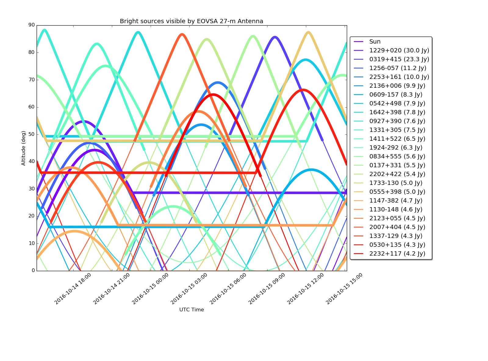
Bin wrote a routine named "eovsa_src_visibility.py" on helios. Dale upgraded it with more user-friendly features named "dg_src_visibility.py". They display the visibility of all VLA calibrators by the 27-m antenna above a certain flux density threshold (defined by parameter "minflux") in C band for a given time and duration. An example of this plot is shown in Fig. 1. From this plot, the observer is asked to create the observing schedule that covers as many calibrator sources as possible, according to some criteria such as: -29d < DEC < 45d, Altitude > 10 deg, and at least 10 ~ 20 deg away from the Sun (etc.?). The observer is advised to include at least one? coverage of the sources 3c286 (1331+305) and 3c48 (0137+331) during the observing schedule.
What to look before/during the observation
Before the schedule start - CryoRX tab
1. Make sure that the first and the second rows (FEMA Outlets and FEMA Receiver) show "ON" and non-zero values. If they aren't, it means that the control system for receiver has died. One way to make it come back is to execute "starburstControl start" in antctl@feanta server (ssh connect from helios). "DrainVoltage" should all be 1.20.
2. RFSwitch: ON - if using high frequency receiver (pcal.fsq), OFF - if using low frequency receiver (pcal_lo.fsq)
3. RXSelect & ZFocus (bottom of FEMA Receiver): "Position" should be [RXSelect,ZFocus] ~[???,7.5?] for the observation using high frequency receiver (pcal.fsq), and ~[103?,28.5?] for the observation using low frequency receiver (pcal_lo.fsq). If you want to change between receiver settings, use "rx-select lo/hi ant14" (change between lo and hi) in Raw Command window. If this command does not switch RXSelect and ZFocus values to the values mentioned earlier, then use "frm-abs-x [target RXSelect position value] ant14" and "frm-abs-z [target ZFocus position value] ant14" for manually setting RXselect & ZFocus position values, respectively. Each target position values should be close to the values mentioned earlier.
Problems expected at the schedule start
Frequency Tuning is not "Sweeping"
1. Try "STOP" and "GO" the schedule
2. If #1 does not work, type "loa1-reboot" in Raw command window
Ant 14(13A) is showing Elevation Permit (the "second column" permit in red)
1. "reboot 1 ant14" - wait 30 seconds until it comes back
2. If you don't want to stop the observation that has already been started, then execute "tracktable pcal_tab.radec ant14" and "track atn14" in Row command window. (change "pcak_tab.radec" part depending on how your schedule is set up accordingly.)
Attenuation
1. Make sure dBm values for both H and V Channels are around 2~3 dB. If not, adjust the attenuation. See Natsuha's write-up about how to change attenuation for how to do it. However, if the source you're observing is weak then the dB values may not reach 2~3 even if attenuation are zeroes. In this case, just leave it. (This might happen for ant 1 and 11.)
2. Ant 14's backend attenuation have to be both 24. For other antennas, the values have to be changing (not every second, but slowly).
During the observation - how to check the phase data of your first file
You can check the phase plots from the files that are stored in DPP right after the first file is created (i.e. 10 minutes after the start of the observation of your first source) to check if things are going okay. It is recommended, though, to check with the source with moderate brightness, which should show good phase data if the observation is going well (e.g. 2136+006, 9.9 Jy).
To check the phase plots, do the following
1. Connect to user@pipeline.solar.pvt (PW is the same for DPP server).
2. Start ipython --pylab.
3. Enter the following commands:
import read_idb as ri
out = ri.read_idb(['the name of your first file'], navg=60)
bl2ord = ri.p.bl_list()
f,ax3 = subplots(4,10)
for k,i in enumerate([the indices of all valid antennas you're observing with]):
    for j in range(4):
        ax3[j,k].plot(angle(out['x'][bl2ord[i,13],0,j]),'.')
        ax3[j,k].set_ylim(-4,4)

4. If there's nothing going wrong with the observation or its setup, then you should see your phase plots being relatively straight over time, like in Figure 2. If not, there could be something wrong, or you could wait another 10 minutes to read the next file to see if it gets better or not.
