Making quick-look flare spectrograms and movies
This page documents instructions for EOVSA Scientists-on-Duty (SoD) to create quicklook flare spectrograms and movies as part of their daily routines.
Prerequisites
Login into the pipeline machine with your account:
ssh -X <your_user_name>@pipeline
If your default shell is not bash, enter bash by
bash
Configuring Access to the Interim Database (IDB)
To process and calibrate EOVSA raw "Interim" Database (IDB) data, access to the SQL database containing the calibration data is required. Perform the following steps to configure access:
Obtain Database Credentials: Contact Bin Chen to request the <username>, <account_name>, and <password> for database access.
Create a ".netrc" File: Create a ".netrc" file in your home directory ("$HOME") with the following contents, replacing "<username>," "<account_name>," and "<password>" with the actual database credentials:
machine eovsa-db0.cgb0fabhwkos.us-west-2.rds.amazonaws.com
           login <username>
           account <account_name>
           password <password>
Secure the ".netrc" File: To ensure that the file is only accessible by you, set its permissions to only allow owner read/write:
chmod 600 ~/.netrc
Set up the Python Environment
If the following is not already in your ~/.bashrc file, do the following
alias loadpyenv3.8='source /home/user/.setenv_pyenv38'
export EOVSADBJSON=/common/python/current/EOVSADB.json
Load the Python 3.8 environment
loadpyenv3.8
ipython --pylab
Producing EOVSA quick-look flare spectrograms
Step 1: Checking Possible flares
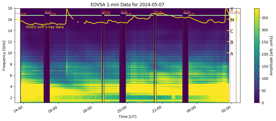
Verify the possible flares on the daily EOVSA Solar Dynamic Spectrogram, for example:
http://ovsa.njit.edu/browser/?suntoday_date=2024-05-07
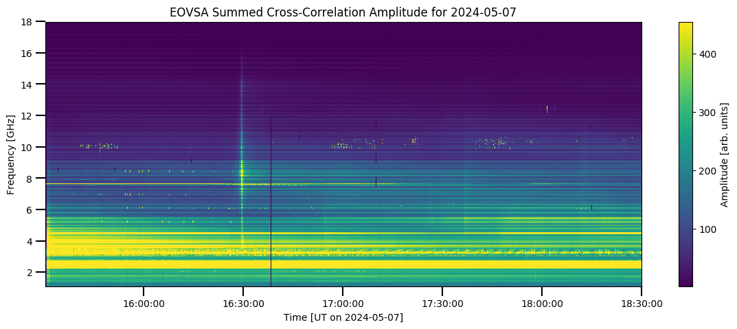
In this example, we see a possible flare that happened around 16:30 UT, which appears as a bright vertical stripe in the daily cross-power dynamic spectrum.
For better visualization and flare time precision, check the higher-resolution dynamic spectra at:
http://ovsa.njit.edu/flaremon/. "XSPYYYYMMDDHHMMSS.png" are the file names you are looking for.
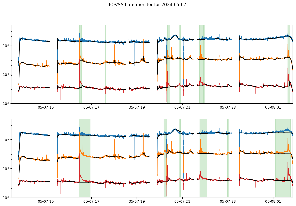
Since 2024-May-05, real-time flare detection figures and list are also available at:
http://ovsa.njit.edu/flaremon/FLM20240507.png http://ovsa.njit.edu/flaremon/flarelist/flarelist_2024-05-07.txt
Step 2: Analyze the flare
Enter a working directory. We have limited space under /home, so it is better to go to your directory under /data1/.
cd /data1/<your_user_name>/
Obtain IDB files by providing a time range that encloses the flare. This step will also perform various calibration steps (absolute flux, attenuator gain, and feed rotation), so it may take a while (a few minutes per file). During the course, it will also ask you to confirm the files to be processed. Each IDB file is supposed to be 10-minute long. The naming convention is "IDByyyymmddhhmmdd," with the time indicating the start time of the file.
In Python, enter the following:
from eovsapy import flare_spec as fs
from eovsapy.util import Time
files = fs.calIDB(Time(['2024-05-07 16:20','2024-05-07 16:35']))
The timerange corresponds to these files (will take about 8 minutes to process)
/data1/eovsa/fits/IDB/20240507/IDB20240507162024
/data1/eovsa/fits/IDB/20240507/IDB20240507163024
Do you want to continue? (say no if you want to adjust timerange) [y/n]?y
The previous step, if successful, will produce a list of IDB files under the current directory
In [21]: print(files)
['./IDB20240507162024', './IDB20240507163024']
Inspect the spectrograms and see if all the antennas look okay.
out, spec_tp, spec_xp, time_axis, freq_axis = fs.inspect(files)
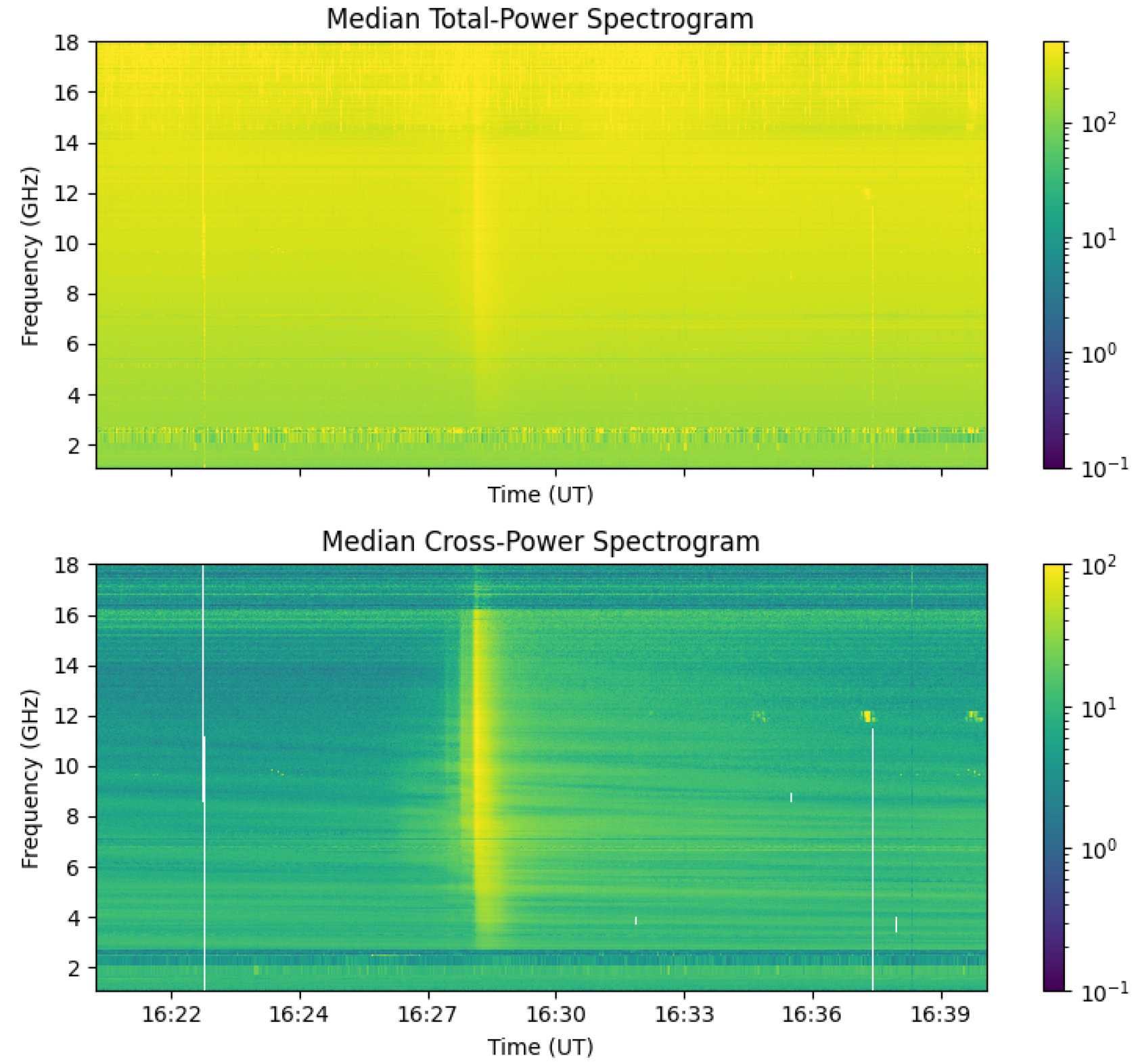
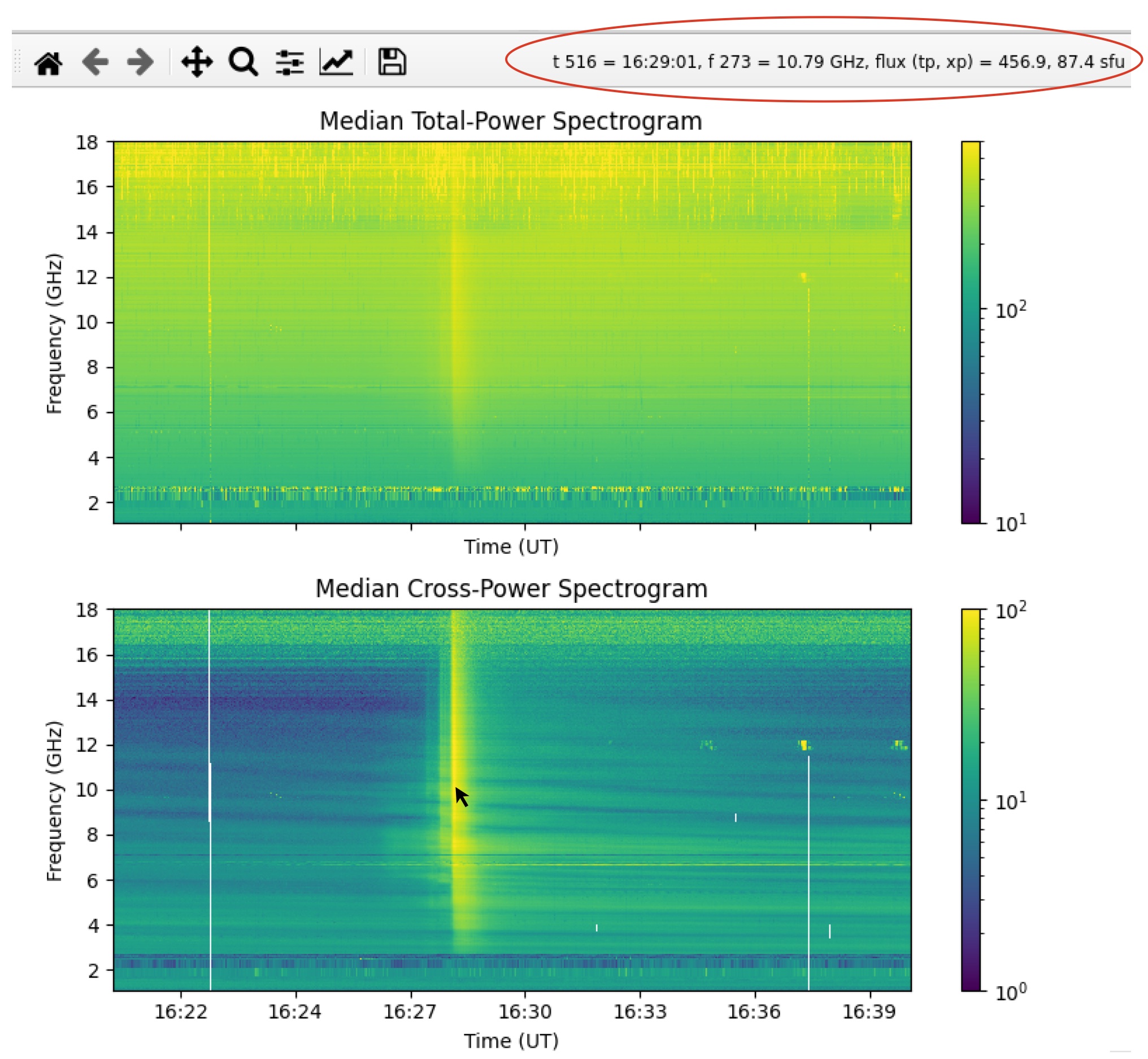
Two figures will be produced. One two-panel figure shows the median total-power spectrogram across all antennas and a cross-power spectrogram across a set of baselines defined by "uvrange" (default to 45 to 300 m).
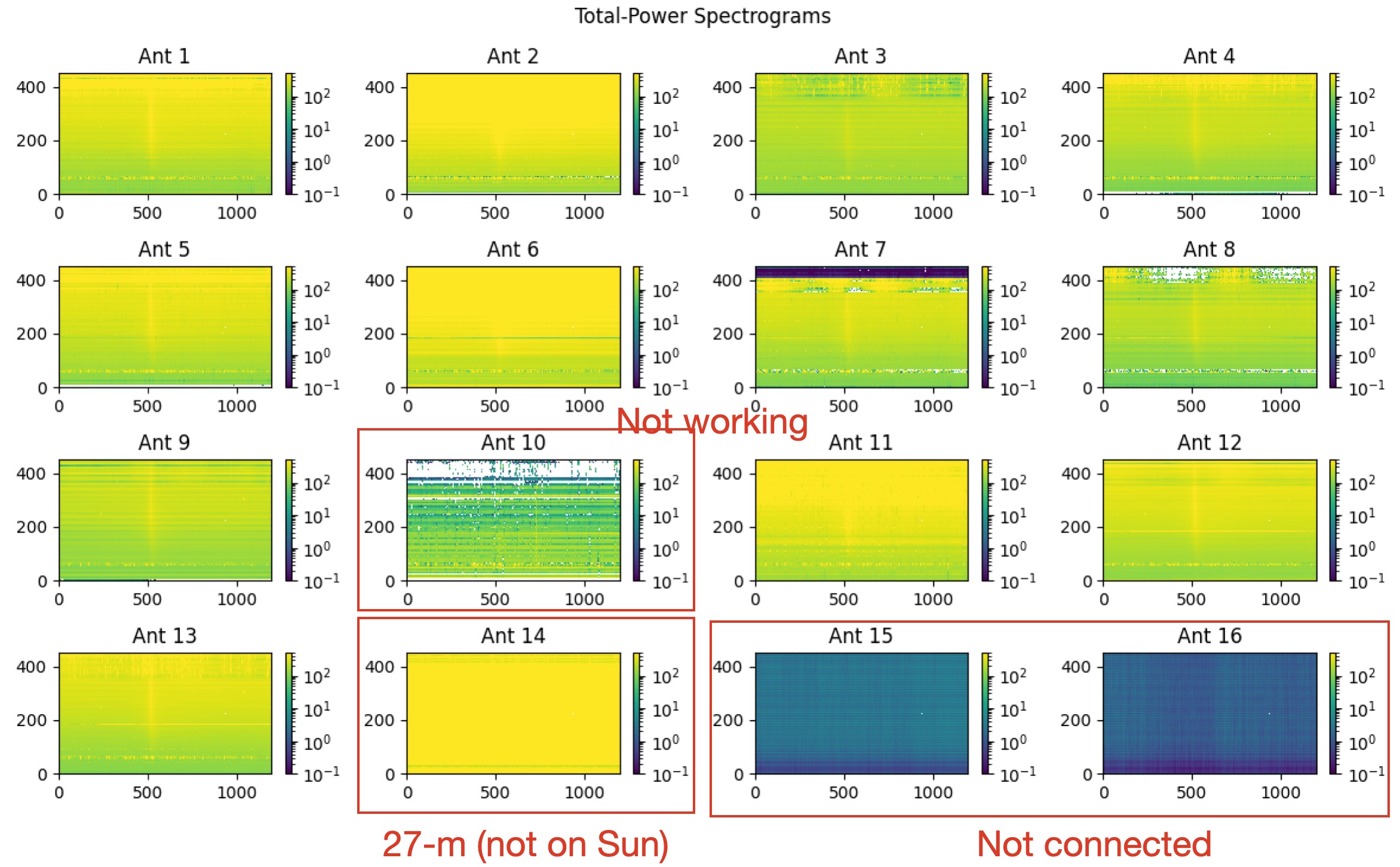
Another shows total-power spectrograms for all 16 antennas. (Note the antenna names go from 1 to 16. Ant 14 is the 27-m for calibrations, and Ants 15 and 16 are not yet connected to the system, but will be available soon.)
To fine-tune the color normalization, you can directly call the plt_quicklook_specs() function by providing spec_tp, spec_xp, and out. Adjust the normalization for the spectrograms using "vmin_tp" and "vmax_tp" for total power and "vmin_xp" and "vmax_xp" for cross power:
fs.plt_quicklook_specs(spec_tp, spec_xp, out=out, vmin_xp=1., vmax_xp=100., vmin_tp=10., vmax_tp=600.)
Check the EOVSA Observing Log for antennas that were not working. We should also check the total-power spectrograms to see if there are any anomalies. In this example, except for Ant 10, all others look okay. However, the observing log says Ant 7 has issues with the Y polarization. Let us exclude both of them using the "ant_str" parameter.
out, spec_tp, spec_xp = fs.inspect(files, ant_str='ant1-6 ant8-9 ant11-13', vmin_xp=1., vmax_xp=100., vmin_tp=10., vmax_tp=600.)
Use the output figure to 1) choose the background interval (bgidx), 2) identify the flare peak time, 3) select frequencies for plotting. The box at the top-right of the plot shows the time index/time string, frequency index/frequency string, flux for total power and cross power at the location of your cursor. Move your cursor around and write the information down. For the background interval, I chose time indices from 170 to 200, as they are close to the flare time, but do not appear to have any flare emission. Also, make sure the range does not have strong RFIs. To reduce the potential of large variations, it is advised to select a background period of more than 10 seconds when possible. The parameter "tpk" is the flare peak time found from EOVSA spectrograms. It determines the name of the resulting files (.png and .fits) and the flare_id. In this example, I found the peak time is very close to 2024-05-07T16:29:01. See the snapshot below. Note the flare peak can vary from frequency to frequency. Let us use 10 GHz as the first reference. If the flare signature at 10 GHz is unclear, use 5 GHz as the second reference. The accuracy of the peak time does not need to be down to the second level. Just use your best judgment.
Step 3: Write out final products
Now, we are ready to make the final products for the spectrograms using the make_plot() function. To ensure the color scaling and antenna/baseline selection are optimized, the cross-power and total-power spectrograms need to be created separately.
Producing final cross-power spectrogram
For the median cross-power spectrogram, our previous selections of the antennas should be fine, as it is a median over many baselines. Also, as we advise to our users, the cross-power spectrograms are not supposed to be used for quantitative spectral analysis but only as a reference for, e.g., timing analysis. So small variations in the flux are okay.
f, ax0, ax1 = fs.make_plot(out, bgidx=[170, 200], vmin=0.1, vmax=110, lcfreqs=[120, 190, 270, 350], ant_str='ant1-6 ant8-9 ant11-13', tpk='2024-05-07 16:29:01', spec_type='xp', writefits=True)
A second background interval can be defined after the flare, if desired. The background will be an interpolation of the two (before and after the flare). e.g., bg2idx=[1000,1010]
In this example, the output files are "eovsa.spec_xp.flare_id_20240507162901.png" and "eovsa.spec_xp.flare_id_20240507162901.fits."
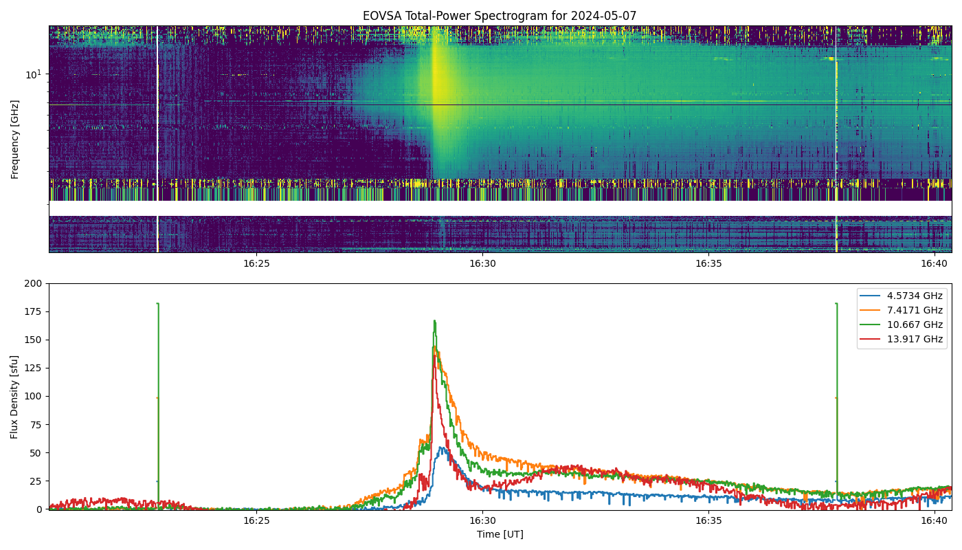
Producing final total-power spectrogram
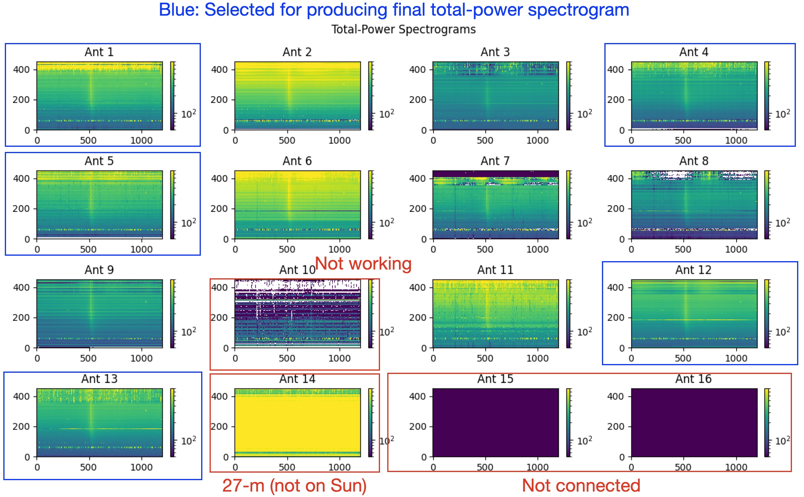
For the total-power spectrum, we need to be more careful. The final product is a median over a number of selected antennas. We need to ensure the total-power spectrograms from these selected antennas are consistent with each other. The exact selection is subjective and varies from observer to observer, but one wants to avoid using antennas that are 1) not working, 2) too noisy, or 3) show significant differences from the others. In this example, I chose antennas 1, 4, 5, 12, and 13, based on the total-power spectrograms plot made by flare_spec.inspect().
f, ax0, ax1 = fs.make_plot(out, bgidx=[170, 220], vmin=1., vmax=200, lcfreqs=[120, 190, 270, 350], ant_str='ant1 ant4 ant5 ant12 ant13', tpk='2024-05-07 16:29:01', spec_type='tp', writefits=True))
At the end, copy the .fits file to /common/webplots/events/2024:
cp eovsa.*.flare_id_20240507162901.* /common/webplots/events/2024
and include the flare in the wiki Flare List:
