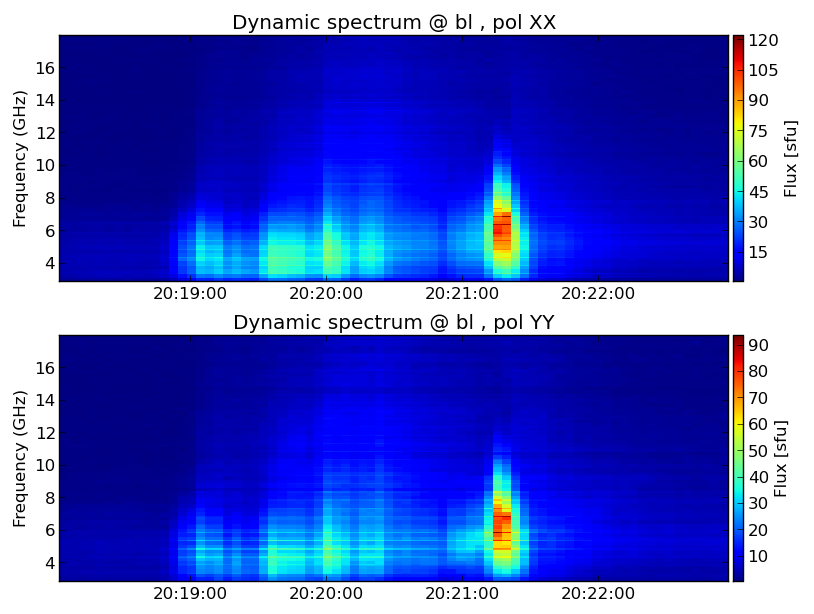
Dynamic Spectrum and Imaging

Overview

This tutorial describes the making dynamic spectrum and imaging the EOVSA microwave data observed on August 21, 2017.

Obtaining the Data

/common/data/eovsa_tutorial/IDB20170821201020-203020.12s.slfcaled.ms on virgo.

Get Dynamic Sepctrum with SunCASA

Within SunCASA, you are using IPython to interact with the system. This does not mean extensive python experience is necessary. Basic Python interactions are straightforward, e.g., assigning parameters, importing modules, running functions. The first module we introduce is dspec. This module allows you to generate a dynamic spectrum from an MS file, and visualize it. You can select a subset of data by specifying a time range, spectral windows/channels, antenna baseline. The selection syntax follows the CASA convention. More information may be found in the CASA guide of time range, spectral windows/channels, antenna baseline selection pages.

Figure 1: EOVSA cross power dynamic spectrum at stokes XX and YY

from suncasa.utils import dspec as ds

# define the visbility data file
msfile = 'IDB20170821201020-203020.12s.slfcaled.ms' 

## define the output filename of the dynamic spectrum 
specfile = msfile + '.dspec.npz'  

##  antenna selection
## leave it blank for selecting all baselines
bl = ''

## Spectral Windows and Channels selection
leave it blank for selecting all spectral windows
spw = ''

## time range selection
## leave it blank for selecting the entire time interval
timeran = ''

## select baselines with a median length (0.2~0.8km)
domedian =True    

## this step generates a dynamic spectrum and saves it to specfile
ds.get_dspec(vis=msfile, specfile=specfile, bl=bl, spw=spw, domedian=domedian)

## this plot the dynamic spectrum.
ds.plt_dspec(specfile, pol='XXYY')

Imaging with SunCASA

cd to your working directory where the measurement sets file is located.

from suncasa.utils import qlookplot as ql
msfile = 'IDB20170821201020-203020.12s.slfcaled.ms'
vis = msfile
timerange = '20:21:10~20:21:30'  ## time range selection
spw = '3.4~6.0GHz'  ## Spectral Windows and Channels selection
stokes = 'XXYY'     ## polarizations selection
ql.qlookplot(vis, timerange=timerange, spw=spw, stokes=stokes)