Tohban EOVSA Imaging Tutorial A-Z
This tutorial describes the step-by-step procedure to download EOVSA IDB data, obtain and calibrate the measurement sets (.ms), and, transfer them to the inti server for self-calibration and further analysis.
Pre-requisites: Accounts on Pipeline and Inti or Baozi servers.
Calibration on your own computer
from suncasa.suncasatasks import calibeovsa
from suncasa.suncasatasks import importeovsa
try:
    # Required in modular casa, but fails in stand-alone casa
    from casatasks import split
except:
    pass
idbfile = <IDB filename>    # The path and filename of the IDB file
msfiles = importeovsa(idbfiles=idbfile)
vis, = calibeovsa(msfiles, caltype=['refpha','phacal'])
outvis = vis.replace('.ms','_cal.ms')
split(vis=vis, outputvis=outvis, correlation='XX')
If all goes well, this will result in a fully-calibrated visibility dataset with the string "_cal.ms" appended to the IDB filename, located in the same place as the original IDB file. You can then start with Step 4 below, for self-calibration.It is now possible to do the entire calibration procedure from anywhere by copying to your local computer one or more raw interim database (IDB) files in Miriad format and calibrating them from a cloud database. Here are the steps. First, find the IDB file(s) of interest. The IDB files are all available online at the following links:
- 2017 Apr - present - 7 days: https://research.ssl.berkeley.edu/data/eovsa/
- 2024 Jan - present: http://ovsa.njit.edu/fits/IDB/
Once you have the file(s) identified for the date and time of interest, copy them to your local computer. One way to do that is with the wget command:
wget -r --no-parent -nH --cut-dirs=3 -e robots="off" -R "index.html*" <URL>
where <URL> is the path to the file(s). For example, to get the data for the flare at 2022 Nov 18 22:04 UT [1] the URL would be http://ovsa.njit.edu/IDB2/20221118/IDB20221118215521/. Warning, these IDB "files" are actually directories, so include the trailing / in the URL or else you will transfer the entire day's data (many GB of data!). An easy way to get the URL is simply to right-click on the web link for the file and "copy link address."
Additional Requirements
Once you have the IDB file downloaded, you will need to add a .netrc in your home directory with the username and password to access the EOVSA cloud database. Please email someone in the NJIT radio group (http://ovsa.njit.edu/people.html) to request that information.
You will also need to install
- the suncasa python package (see the readme file at https://github.com/suncasa/suncasa-src for complete installation instructions),
- the eovsapy python package (see https://github.com/suncasa/eovsapy for installation instructions).
Calibration on the Pipeline computer at OVRO
Connection details to pipeline server
One can use the Mobaxterm platform to connect to the Pipeline server through a Windows machine or use SSH through a Mac machine.
Step 0: First time pipeline environment setup
First time users of pipelines ipython environment should
1. add the following line to ~/.bashrc (ex /home/shaheda/.bashrc not in your /data1/ folder)
alias loadpyenv3.8='source /home/user/.setenv_pyenv38'
2. run the following line
cp /home/user/.netrc ~/
Step 1: Importing to CASA from raw data (IDB) on the Pipeline machine
In Python on the Pipeline machine, which has the complete EOVSA SQL database. (bash; load pyenv3.8; ipython)
If you are not using mobaxterm, directly SSH to Pipeline through your Linux or Mac computer.
from suncasa.suncasatasks import calibeovsa
from suncasa.suncasatasks import importeovsa
from casatasks import split
from eovsapy.read_idb import get_trange_files
from eovsapy.util import Time
import numpy as np
import os

trange = Time(['2017-08-21 20:15:00', '2017-08-21 20:35:00'])                               ###Change accordingly###
files = get_trange_files(trange)

outpath = './msdata/'                                                                       ###Change accordingly###
if not os.path.exists(outpath):
    os.makedirs(outpath)

msfiles = importeovsa(idbfiles=files, ncpu=1, timebin="0s", width=1,
                                   visprefix=outpath,
                                   nocreatms=False, doconcat=False,
                                   modelms="", doscaling=False, keep_nsclms=False, udb_corr=True)
If you come across errors with calibeovsa, add following lines to your ~/.casa/init.py file.
import sys
sys.path.append('/common/python')
sys.path.append('/common/python/packages/pipeline_casa')
execfile('/common/python/suncasa/tasks/mytasks.py')
Step 2: Concatenate all the 10 mins data, if there are any
Follow this step if there are more than one .ms files, if not run step 3 directly. If doimage=True, a quicklook image will be produced (by integrating over the entire time) as shown below. If Step 2 is used, skip the calibeovsa in Step 3 (you already did it when you concat)
# This is to set the path/name for the concatenated files
concatvis = os.path.basename(msfiles[0])[:11] + '_concat_cal.ms'
vis = calibeovsa(msfiles, doconcat=True, concatvis=concatvis, caltype=['refpha','phacal'], doimage=False)
Step 3: Calibration
This will calibrate the input visibility, write out calibration tables under /data1/eovsa/caltable/, and apply the calibration.
vis = calibeovsa(msfiles, caltype=['refpha','phacal'], doimage=False)            ###Change the vis filename accordingly###
# Append '_cal' to the ms filename and split the corrected column to the new caled ms
vis_str = str(' '.join(vis))
caled_vis=vis_str.replace('.ms','_cal.ms')
split(vis=' '.join(vis),outputvis=caled_vis,datacolumn='corrected',timerange='',correlation='XX')
One needs to transfer the created caled ms data files (xxx_concat_cal.ms or xxx_cal.ms) from pipeline to inti server, which has all the casatasks installed, in order to run the rest of the imaging steps.
Connection details to Inti server
For Windows, on Mobaxterm,
- With your NJIT VPN connected, connect to one of the afsconnect servers (for example, afsaccess3.njit.edu) using your UCID and password.
- ssh -X UCID@inti.hpcnet.campus.njit.edu
To avoid typing the full inti address each time you attempt for ssh, you may wish to add the following lines with your username to C:\Program Files\Git\etc\ssh\ssh_config on Windows and /.ssh/config on Mac and Linux machines.
Host inti
Hostname inti.hpcnet.campus.njit.edu
User USERNAME                                                                                              ###Insert UCID/inti username here###
To have sufficient disk space with EOVSA data analysis over Inti, use your dedicated directory YOURDIRECTORY at the location given below. If you do not have a directory, Please take help from Sijie in creating one.
cd /inti/data/users/YOURDIRECTORY
For Linux or Mac machine, ssh -X UCID@inti.hpcnet.campus.njit.edu
Transferring data files between servers
For directly transferring your calibrated .ms data between the Pipeline and Inti servers, follow the below given steps.
1. Log into Inti using your username.
ssh -X USERNAME@inti.hpcnet.campus.njit.edu

Then create a tunnel into Pipeline from Inti.
ssh -L 8888:pipeline.solar.pvt:22 guest@ovsa.njit.edu

2. Log into Inti again from a new terminal.

Change to your working directory and give this command to copy your data on Pipeline.
scp -v -C -r -P 8888 USERNAMEofPipeline@localhost:PATHofMSDATA/MSfilename ./
Eg: scp -v -C -r -P 8888 shaheda@localhost:/data1/shaheda/IDB20220118173922_cal.ms ./
where, MSfilename, PATHofMSDATA are your .ms data and its path on Pipeline machine.
Alternatively, one can follow the below procedure to do the transfer.
For Windows, on mobaxterm, drag and drop the ms file to your local machine or use scp command as given below.
scp -r -C userid@pipeline:/your/folder/msfile /localmachine/destination/folder/
On mobaxterm and on your local terminal, use the following command to finally copy the ms file to Inti.
scp -r -C /localmachine/destination/folder/msfile UCID@inti.hpcnet.campus.njit.edu:/inti/data/users/YOURDIRECTORY
For Mac and Linux, SCP can be used in the same way. Add the following lines to your SSH config file, to bypass ovsa.njit.edu from copying. vi ~/.ssh/config
Host ovsa
        HostName ovsa.njit.edu
        User guest
Host pipeline
        Hostname pipeline.solar.pvt
        User userid
        ProxyCommand ssh -W %h:%p guest@ovsa.njit.edu
Software details on the servers
On Inti, when logging in for the first time, please add the following lines to your accounts ~/.bashrc file.
>>vi ~/.bashrc Insert the text given below and save it.
#### setting start ####
if [ $HOSTNAME == "baozi.hpcnet.campus.njit.edu" ]; then
    source /srg/.setenv_baozi
fi
if [ $HOSTNAME == "inti.hpcnet.campus.njit.edu" ]; then
    source /inti/.setenv_inti
fi
if [ $HOSTNAME == "guko.resource.campus.njit.edu" ]; then
    source /data/data/.setenv_guko
fi
#### setting end ####
Both CASA 5 and 6 are available on Inti.
Enter the bash environment on inti, and load the desired casa environment. To load CASA 5, enter bash environment by giving >>bash
>> loadcasa5
>> suncasa              #This should load the software making you ready for the analysis
Or to load CASA 6, enter bash environment by giving >>bash
>> loadcasa6
>> ipython              #This should load the software making you ready for the analysis
Here, for example, to use clean, first start ipython as given above, then type in >>from casatasks import tclean
Step 4: Self-calibration

Follow the below given steps to run the self-calibration of the imaging data and produce the calibrated images in .fits format. https://github.com/binchensun/casa-eovsa/blob/master/slfcal_example.py
from suncasa.utils import helioimage2fits as hf
import os
import numpy as np
import pickle
from matplotlib import gridspec as gridspec
from sunpy import map as smap
from matplotlib import pyplot as plt
from split_cli import split_cli as split
import time

# =========== task handlers =============
dofullsun = 1 # initial full-sun imaging                                         ###Change accordingly###
domasks=1 # get masks                                                            ###Change accordingly###
doslfcal=1 # main cycle of doing selfcalibration                                 ###Change accordingly###
doapply=1 # apply the results                                                    ###Change accordingly###
doclean_slfcaled=1 # perform clean for self-calibrated data                      ###Change accordingly###

# ============ declaring the working directories ============
workdir = os.getcwd()+'/' #main working directory. Using current directory in this example
slfcaldir = workdir+'slfcal/' #place to put all selfcalibration products
imagedir = slfcaldir+'images/' #place to put all selfcalibration images
maskdir = slfcaldir+'masks/' #place to put clean masks
imagedir_slfcaled = slfcaldir+'images_slfcaled/' #place to put final self-calibrated images
caltbdir = slfcaldir+'caltbs/' # place to put calibration tables
# make these directories if they do not already exist
dirs = [workdir, slfcaldir, imagedir, maskdir, imagedir_slfcaled, caltbdir]
for d in dirs:
    if not os.path.exists(d):
        os.makedirs(d)

# ============ Split a short time for self-calibration ===========
# input visibility
ms_in = workdir + 'IDB20170821202020_cal.ms'                                    ###Change the initial calibrated (through calibeovsa) vis accordingly###
# output, selfcaled, visibility
ms_slfcaled = workdir + os.path.basename(ms_in).replace('cal','slfcaled')
# intermediate small visibility for selfcalbration
# selected time range for generating self-calibration solutions
trange='2017/08/21/20:21:10~2017/08/21/20:21:30'                                ###Change accordingly###
slfcalms = slfcaldir+'slfcalms.XX.slfcal'
slfcaledms = slfcaldir+'slfcalms.XX.slfcaled'
if not os.path.exists(slfcalms):
    split(vis=ms_in,outputvis=slfcalms,datacolumn='data',timerange=trange,correlation='XX')

# ============ Prior definitions for spectral windows, antennas, pixel numbers =========
spws=[str(s+1) for s in range(30)]                                              ###spws=[str(s+1) for s in range(49)]   # For post-2020 data
antennas='0~12&0~12'
npix=512
nround=3 #number of slfcal cycles
4.1
# =========== Step 1, doing a full-Sun image to find out phasecenter and appropriate field of view =========
if dofullsun:
    #initial mfs clean to find out the image phase center
    im_init='fullsun_init'
    os.system('rm -rf '+im_init+'*')
    tclean(vis=slfcalms,
            antenna=antennas,
            imagename=im_init,
            spw='1~15',
            specmode='mfs',
            timerange=trange,
            imsize=[npix],
            cell=['5arcsec'],
            niter=1000,
            gain=0.05,
            stokes='I',
            restoringbeam=['30arcsec'],
            interactive=False,
            pbcor=True)

    hf.imreg(vis=slfcalms,imagefile=im_init+'.image.pbcor',fitsfile=im_init+'.fits',
             timerange=trange,usephacenter=False,verbose=True)
    clnjunks = ['.flux', '.mask', '.model', '.psf', '.residual','.sumwt','.pb','.image']     #Do not run the next 4 lines if needed to view and assess the subset of clean process images
    for clnjunk in clnjunks:
        if os.path.exists(im_init + clnjunk):
            os.system('rm -rf '+im_init + clnjunk)

    from sunpy import map as smap
    from matplotlib import pyplot as plt
    fig = plt.figure(figsize=(6,6))
    ax = fig.add_subplot(111)
    eomap=smap.Map(im_init+'.fits')
    #eomap.data=eomap.data.reshape((npix,npix))
    eomap.plot_settings['cmap'] = plt.get_cmap('jet')
    eomap.plot(axes = ax)
    eomap.draw_limb()
    plt.show()
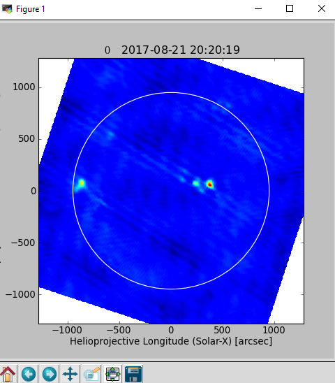
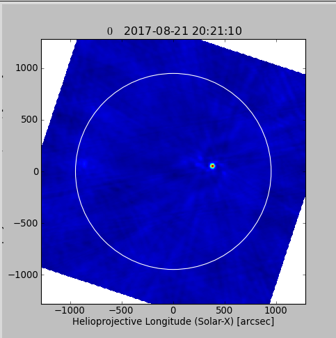
    viewer(im_init+'.image.pbcor')
4.2
# parameters specific to the event (found from step 1)
phasecenter='J2000 10h02m59 11d58m07'                                               ###Change accordingly###
xran=[280,480]                                                                      ###Change accordingly###
yran=[-50,150]                                                                      ###Change accordingly###


# =========== Step 2 (optional), generate masks =========
# if skipped, will not use any masks
if domasks:
    clearcal(slfcalms)
    delmod(slfcalms)
    antennas=antennas
    pol='XX'
    imgprefix=maskdir+'slf_t0'

    # step 1: set up the clean masks
    img_init=imgprefix+'_init_ar_'
    os.system('rm -rf '+img_init+'*')
    #spwrans_mask=['1~5','6~12','13~20','21~30']
    spwrans_mask=['1~12']
    #convert to a list of spws
    spwrans_mask_list = [[str(i) for i in (np.arange(int(m.split('~')[0]),int(m.split('~')[1])))] for m in spwrans_mask]   # Not used?
    masks=[]
    imnames=[]
    for spwran in spwrans_mask:
        imname=img_init+spwran.replace('~','-')
        try:
            tclean(vis=slfcalms,
                    antenna=antennas,
                    imagename=imname,
                    spw=spwran,
                    specmode='mfs',
                    timerange=trange,
                    imsize=[npix],
                    cell=['2arcsec'],
                    niter=1000,
                    gain=0.05,
                    stokes='XX',
                    restoringbeam=['20arcsec'],
                    phasecenter=phasecenter,
                    weighting='briggs',
                    robust=1.0,
                    interactive=True,
		    datacolumn='data',
                    pbcor=True,
                    savemodel='modelcolumn')
            imnames.append(imname+'.image')
            masks.append(imname+'.mask')
            clnjunks = ['.flux', '.model', '.psf', '.residual']   #Do not run the next 4 lines if needed to view and assess the subset of clean process images
            for clnjunk in clnjunks:
                if os.path.exists(imname + clnjunk):
                    os.system('rm -rf '+ imname + clnjunk)
        except:
            print('error in cleaning spw: '+spwran)

    pickle.dump(masks,open(slfcaldir+'masks.p','wb'))
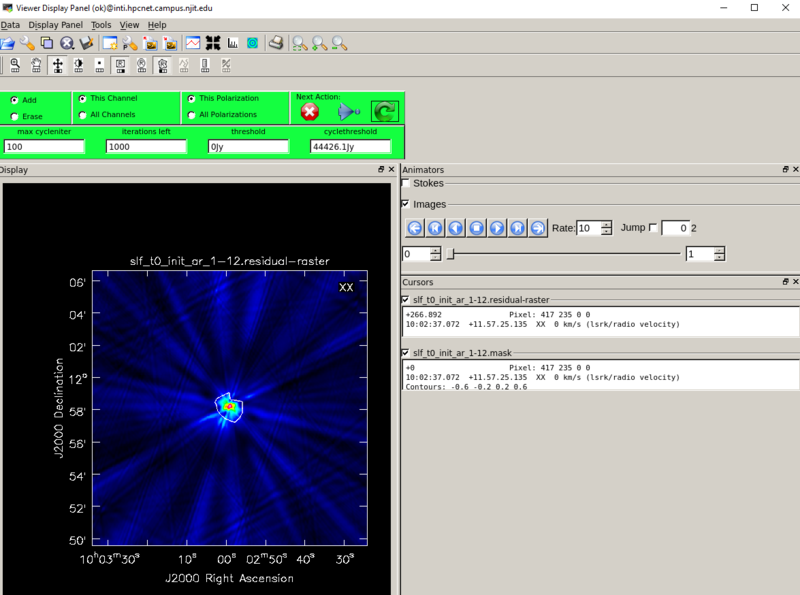
The outlines drawn for masks can be created by any of the icons with the letter 'R' in the Viewer window. The instructions for doing this can be found by hovering over those icons.
4.3
# =========== Step 3, main step of selfcalibration =========
if doslfcal:
    if os.path.exists(slfcaldir+'masks.p'):
        masks=pickle.load(open(slfcaldir+'masks.p','rb'))
    if not os.path.exists(slfcaldir+'masks.p'):
        print 'masks do not exist. Use default mask'
        masks=[]
    os.system('rm -rf '+imagedir+'*')
    os.system('rm -rf '+caltbdir+'*')
    #first step: make a mock caltable for the entire database
    print('Processing ' + trange)
    slftbs=[]
    calprefix=caltbdir+'slf'
    imgprefix=imagedir+'slf'
    tb.open(slfcalms+'/SPECTRAL_WINDOW')
    reffreqs=tb.getcol('REF_FREQUENCY')
    bdwds=tb.getcol('TOTAL_BANDWIDTH')
    cfreqs=reffreqs+bdwds/2.
    tb.close()
    # starting beam size at 3.4 GHz in arcsec        #Change accordingly
    sbeam=40.
    strtmp=[m.replace(':','') for m in trange.split('~')]
    timestr='t'+strtmp[0]+'-'+strtmp[1]
    refantenna='0'
    # number of iterations for each round
    niters=[100, 300, 500]
    # roburst value for weighting the baselines
    robusts=[1.0, 0.5, 0.0]
    # apply calibration tables? Set to true for most cases
    doapplycal=[1,1,1]
    # modes for calibration, 'p' for phase-only, 'a' for amplitude only, 'ap' for both
    calmodes=['p','p','a']
    # setting uvranges for model image (optional, not used here)
    uvranges=['','','']
    for n in range(nround):
        slfcal_tb_g= calprefix+'.G'+str(n)
        fig = plt.figure(figsize=(8.4,7.))                                 # fig = plt.figure(figsize=(14, 7))   # For post-2020 data (50 spws)
        gs = gridspec.GridSpec(5, 6)                                       # gs = gridspec.GridSpec(5, 10)        # For post-2020 data (50 spws)
        for s,sp in enumerate(spws):
            print 'processing spw: '+sp
            cfreq=cfreqs[int(sp)]
            # setting restoring beam size (not very useful for selfcal anyway, but just to see the results)
            bm=max(sbeam*cfreqs[1]/cfreq, 6.)
            slfcal_img = imgprefix+'.spw'+sp.zfill(2)+'.slfcal'+str(n)
            # only the first round uses nearby spws for getting initial model
            if n == 0:
                spbg=max(int(sp)-2,1)                                      # spbg=max(int(sp)-2,0)               # For post-2020 data (50 spws)
                sped=min(int(sp)+2,30)                                     # sped=min(int(sp)+2,49)              # For post-2020 data (50 spws)
                spwran=str(spbg)+'~'+str(sped)
                print('using spw {0:s} as model'.format(spwran))
                if 'spwrans_mask' in vars():
                    for m, spwran_mask in enumerate(spwrans_mask):
                        if sp in spwran_mask:
                            mask = masks[m]
                            print('using mask {0:s}'.format(mask))
                            findmask = True
                    if not findmask:
                        print('mask not found. Do use any masks')
            else:
                spwran = sp
                if 'spwrans_mask' in vars():
                    for m, spwran_mask in enumerate(spwrans_mask):
                        if sp in spwran_mask:
                            mask = masks[m]
                            print 'using mask {0:s}'.format(mask)
                            findmask = True
                    if not findmask:
                        print('mask not found. Do use any masks')
            try:
                tclean(vis=slfcalms,
                        antenna=antennas,
                        imagename=slfcal_img,
                        uvrange=uvranges[n],
                        spw=spwran,
                        specmode='mfs',
                        timerange=trange,
                        imsize=[npix],
                        cell=['2arcsec'],
                        niter=niters[n],
                        gain=0.05,
                        stokes='XX', #use pol XX image as the model
                        weighting='briggs',
                        robust=robusts[n],
                        phasecenter=phasecenter,
                        mask=mask,
                        restoringbeam=[str(bm)+'arcsec'],
                        pbcor=False,
                        interactive=False,
                        savemodel='modelcolumn')
                if os.path.exists(slfcal_img+'.image'):
                    fitsfile=slfcal_img+'.fits'
                    hf.imreg(vis=slfcalms,imagefile=slfcal_img+'.image',fitsfile=fitsfile,
                             timerange=trange,usephacenter=False,toTb=True,verbose=False,overwrite=True)
                clnjunks = ['.mask','.flux', '.model', '.psf', '.residual', '.image','.pb','.image.pbcor','.sumwt']   #Do not run the next 4 lines if needed to view and assess the subset of clean process images
                for clnjunk in clnjunks:
                    if os.path.exists(slfcal_img + clnjunk):
                        os.system('rm -rf '+ slfcal_img + clnjunk)
                ax = fig.add_subplot(gs[s])
                eomap=smap.Map(fitsfile)
                eomap.plot_settings['cmap'] = plt.get_cmap('jet')
                eomap.plot(axes = ax)
                eomap.draw_limb()
                #eomap.draw_grid()
                ax.set_title(' ')
		ax.get_xaxis().set_visible(False)
		ax.get_yaxis().set_visible(False)
                ax.set_xlim(xran)
                ax.set_ylim(yran)
                plt.pause(0.5)                           # Allows viewing of each image as it is plotted.
                os.system('rm -f '+ fitsfile)

            except:
                print 'error in cleaning spw: '+sp
                print 'using nearby spws for initial model'
                sp_e=int(sp)+2
                sp_i=int(sp)-2
                if sp_i < 1:                              # if sp < 0:                           # For post-2020 data (50 spws)
                    sp_i = 1                              #     sp_i = 0                         # For post-2020 data (50 spws)
                if sp_e > 30:                             # if sp_e > 49:                        # For post-2020 data (50 spws)
                    sp_e = 30                             #     sp_e = 49                        # For post-2020 data (50 spws)
                sp_=str(sp_i)+'~'+str(sp_e)
                try:
                    tget(tclean)
                    spw=sp_
                    print('using spw {0:s} as model'.format(sp_))
                    tclean()
                except:
                    print 'still not successful. abort...'
                    break

            gaincal(vis=slfcalms, refant=refantenna,antenna=antennas,caltable=slfcal_tb_g,spw=sp, uvrange='',\
                    gaintable=[],selectdata=True,timerange=trange,solint='inf',gaintype='G',calmode=calmodes[n],\
                    combine='',minblperant=4,minsnr=2,append=True)
            if not os.path.exists(slfcal_tb_g):
                print 'No solution found in spw: '+sp
        figname=imagedir+'slf_t0_n{:d}.png'.format(n)
	plt.subplots_adjust(left=0, bottom=0, right=1, top=1, wspace=0, hspace=0)
        plt.savefig(figname)
        time.sleep(10)
        plt.close()

        if os.path.exists(slfcal_tb_g):
            slftbs.append(slfcal_tb_g)
            slftb=[slfcal_tb_g]
            os.chdir(slfcaldir)
            if calmodes[n] == 'p':
                plotcal(caltable=slfcal_tb_g,antenna='1~12',xaxis='freq',yaxis='phase',\
                        subplot=431,plotrange=[-1,-1,-180,180],iteration='antenna',figfile=slfcal_tb_g+'.png',showgui=False)
            if calmodes[n] == 'a':
                plotcal(caltable=slfcal_tb_g,antenna='1~12',xaxis='freq',yaxis='amp',\
                        subplot=431,plotrange=[-1,-1,0,2.],iteration='antenna',figfile=slfcal_tb_g+'.png',showgui=False)
            os.chdir(workdir)
            plt.pause(0.5)                               # Allows viewing of the plot

        if doapplycal[n]:
            clearcal(slfcalms)
            delmod(slfcalms)
            applycal(vis=slfcalms,gaintable=slftb,spw=','.join(spws),selectdata=True,\
                     antenna=antennas,interp='nearest',flagbackup=False,applymode='calonly',calwt=False)

        if n < nround-1:
            prompt=raw_input('Continuing to selfcal?')
            #prompt='y'
            if prompt.lower() == 'n':
                if os.path.exists(slfcaledms):
                    os.system('rm -rf '+slfcaledms)
                split(slfcalms,slfcaledms,datacolumn='corrected')
                print 'Final calibrated ms is {0:s}'.format(slfcaledms)
                break
            if prompt.lower() == 'y':
                slfcalms_=slfcalms+str(n)
                if os.path.exists(slfcalms_):
                    os.system('rm -rf '+slfcalms_)
                split(slfcalms,slfcalms_,datacolumn='corrected')
                slfcalms=slfcalms_
        else:
            if os.path.exists(slfcaledms):
                os.system('rm -rf '+slfcaledms)
            split(slfcalms,slfcaledms,datacolumn='corrected')
            print 'Final calibrated ms is {0:s}'.format(slfcaledms)
4.4
# =========== Step 4: Apply self-calibration tables =========
if doapply:
    import glob
    os.chdir(workdir)
    clearcal(ms_in)
    clearcal(slfcalms)
    applycal(vis=slfcalms,gaintable=slftbs,spw=','.join(spws),selectdata=True,\
             antenna=antennas,interp='linear',flagbackup=False,applymode='calonly',calwt=False)
    applycal(vis=ms_in,gaintable=slftbs,spw=','.join(spws),selectdata=True,\
             antenna=antennas,interp='linear',flagbackup=False,applymode='calonly',calwt=False)
    if os.path.exists(ms_slfcaled):
        os.system('rm -rf '+ms_slfcaled)
    split(ms_in, ms_slfcaled,datacolumn='corrected')
4.5
# =========== Step 5: Generate final self-calibrated images (optional) =========
if doclean_slfcaled:
    import glob
    pol='XX'
    print('Processing ' + trange)
    img_final=imagedir_slfcaled+'/slf_final_{0}_t0'.format(pol)
    vis = ms_slfcaled
    tb.open(vis+'/SPECTRAL_WINDOW')
    reffreqs=tb.getcol('REF_FREQUENCY')
    bdwds=tb.getcol('TOTAL_BANDWIDTH')
    cfreqs=reffreqs+bdwds/2.
    tb.close()
    sbeam=30.
    from matplotlib import gridspec as gridspec
    from sunpy import map as smap
    from matplotlib import pyplot as plt
    fitsfiles=[]
    for s,sp in enumerate(spws):
        cfreq=cfreqs[int(sp)]
        bm=max(sbeam*cfreqs[1]/cfreq,4.)
        imname=img_final+'_s'+sp.zfill(2)
        fitsfile=imname+'.fits'
        if not os.path.exists(fitsfile):
            print 'cleaning spw {0:s} with beam size {1:.1f}"'.format(sp,bm)
            try:
                tclean(vis=vis,
                        antenna=antennas,
                        imagename=imname,
                        spw=sp,
                        specmode='mfs',
                        timerange=trange,
                        imsize=[npix],
                        cell=['1arcsec'],
                        niter=1000,
                        gain=0.05,
                        stokes=pol,
                        weighting='briggs',
                        robust=2.0,
                        restoringbeam=[str(bm)+'arcsec'],
                        phasecenter=phasecenter,
                        mask='',
                        pbcor=True,
                        interactive=False)
            except:
                print 'cleaning spw '+sp+' unsuccessful. Proceed to next spw'
                continue
            if os.path.exists(imname+'.image.pbcor'):
                imn = imname+'.image.pbcor'
                hf.imreg(vis=vis,imagefile=imn,fitsfile=fitsfile,
                         timerange=trange,usephacenter=False,toTb=True,verbose=False)
            fitsfiles.append(fitsfile)
            junks=['.flux','.model','.psf','.residual','.mask','.image','.pb','.image.pbcor','.sumwt']  #Do not run the next 4 lines if needed to view and assess the subset of clean process images
            for junk in junks:
                if os.path.exists(imname+junk):
                    os.system('rm -rf '+imname+junk)
        else:
            print('fits file '+fitsfile+' already exists, skip clean...')
            fitsfiles.append(fitsfile)

    fig = plt.figure(figsize=(8.4,7.))                             # fig = plt.figure(figsize=(14, 7))   # For post-2020 data (50 spws)
    gs = gridspec.GridSpec(5, 6)                                   # gs = gridspec.GridSpec(5, 10)       # For post-2020 data (50 spws)
    for s,sp in enumerate(spws):
        cfreq=cfreqs[int(sp)]
        ax = fig.add_subplot(gs[s])
        eomap=smap.Map(fitsfiles[s])
        eomap.plot_settings['cmap'] = plt.get_cmap('jet')
        eomap.plot(axes = ax)
        eomap.draw_limb()
        ax.set_title(' ')
        ax.get_xaxis().set_visible(False)
        ax.get_yaxis().set_visible(False)
        ax.set_xlim(xran)
        ax.set_ylim(yran)
        plt.text(0.98,0.85,'{0:.1f} GHz'.format(cfreq/1e9),transform=ax.transAxes,ha='right',color='w',fontweight='bold')
    plt.subplots_adjust(left=0, bottom=0, right=1, top=1, wspace=0, hspace=0)
    plt.show()
The .fits files of the self calibrated images at each frequency for the given time are saved at /slfcal/images_slfcaled in your working directory.
Step 5: Quick-look imaging
For spectral imaging analysis of the event, follow this tutorial using the self-calibrated data obtained from the previous step or use this link.
from suncasa.utils import qlookplot as ql    ## (Optional) Supply the npz file of the dynamic spectrum from previous step.
				            ## If not provided, the program will generate a new one from the visibility.
                                            ## set the time interval
from suncasa import dspec as ds
import time
visibility_data = 'IDB20170821202020_slfcaled.ms'
specfile = visibility_data + '.dspec.npz'
d = ds.Dspec(visibility_data, bl='4&9', specfile=specfile)

timerange = '19:02:00~19:02:10'             ## select frequency range from 2.5 GHz to 3.5 GHz
spw = '2~5'                                 ## select stokes XX
stokes = 'XX'                               ## turn off AIA image plotting, default is True
plotaia = False
xycen = [375, 45]  ## image center for clean in solar X-Y in arcsec
cell=['2.0arcsec'] ## pixel size
imsize=[128]   ## x and y image size in pixels.
fov = [100,100]  ## field of view of the zoomed-in panels in unit of arcsec
spw = ['{}'.format(s) for s in range(1,31)]
clevels = [0.5, 1.0]  ## contour levels to fill in between.
calpha=0.35  ## now tune down the alpha
restoringbeam=['6arcsec']
ql.qlookplot(vis=msfile, specfile=specfile, timerange=timerange, spw=spw, stokes=stokes, \
            restoringbeam=restoringbeam,imsize=imsize,cell=cell, \
            xycen=xycen,fov=fov,clevels=clevels,calpha=calpha)


