EOVSA Data Products

Introduction

The Expanded Owens Valley Solar Array (EOVSA) observes the full solar disk whenever the Sun is more than 10 degrees above the local horizon. Depending on season, the observing day is approximately 7--12 hours long and is centered near 20 UT. EOVSA records 451 science frequency channels each second in four polarization products, together with total-power measurements from individual antennas.

This page describes the maintained data products and the current access workflow. The authoritative public entry point is the EOVSA Data Browser. Product availability varies with observing date and processing version.

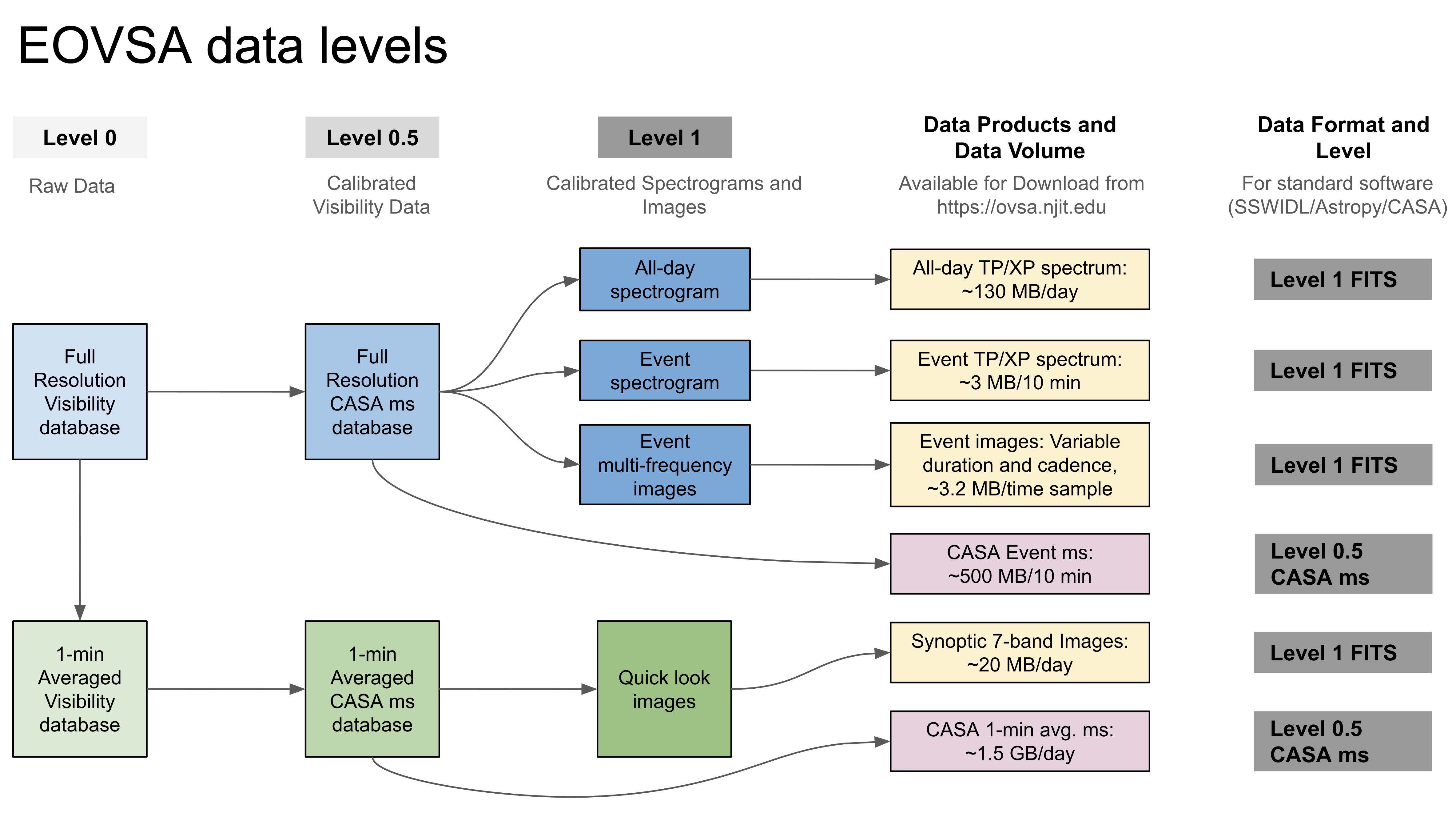
Start here: EOVSA Data Browser

Use the EOVSA Data Browser as the main entry point for finding, previewing, and downloading Level 1 EOVSA data. Select an observing date in UTC, or use Coverage to find dates with imaging or spectrogram products. Product previews and the flare list can be explored before signing in; registration by email is required when downloading data files.

For a guided introduction, select the Tour button in the site header. The on-page tour walks through the date and coverage controls, image viewer, product downloads, spectrograms, flare table, and interactive flare plot.

Site area	What is provided	How to use it
Spectrograms	A daily 1-minute EOVSA summary, a selectable full-resolution TP or XP spectrogram preview, and a multi-instrument context summary.	Select a UTC date and scroll to Spectrograms. Switch between TP and XP. Full-day TP/XP FITS files are available through Product Downloads when present.
Synoptic maps	Full-disk views in seven EOVSA bands, an all-bands overview, a focused single-band view, and the synoptic imaging product versions available for that date.	Select an EOVSA band and Product Version in the Image Viewer. Use Product Downloads for daily or sequence products in FITS, and JP2 when available.
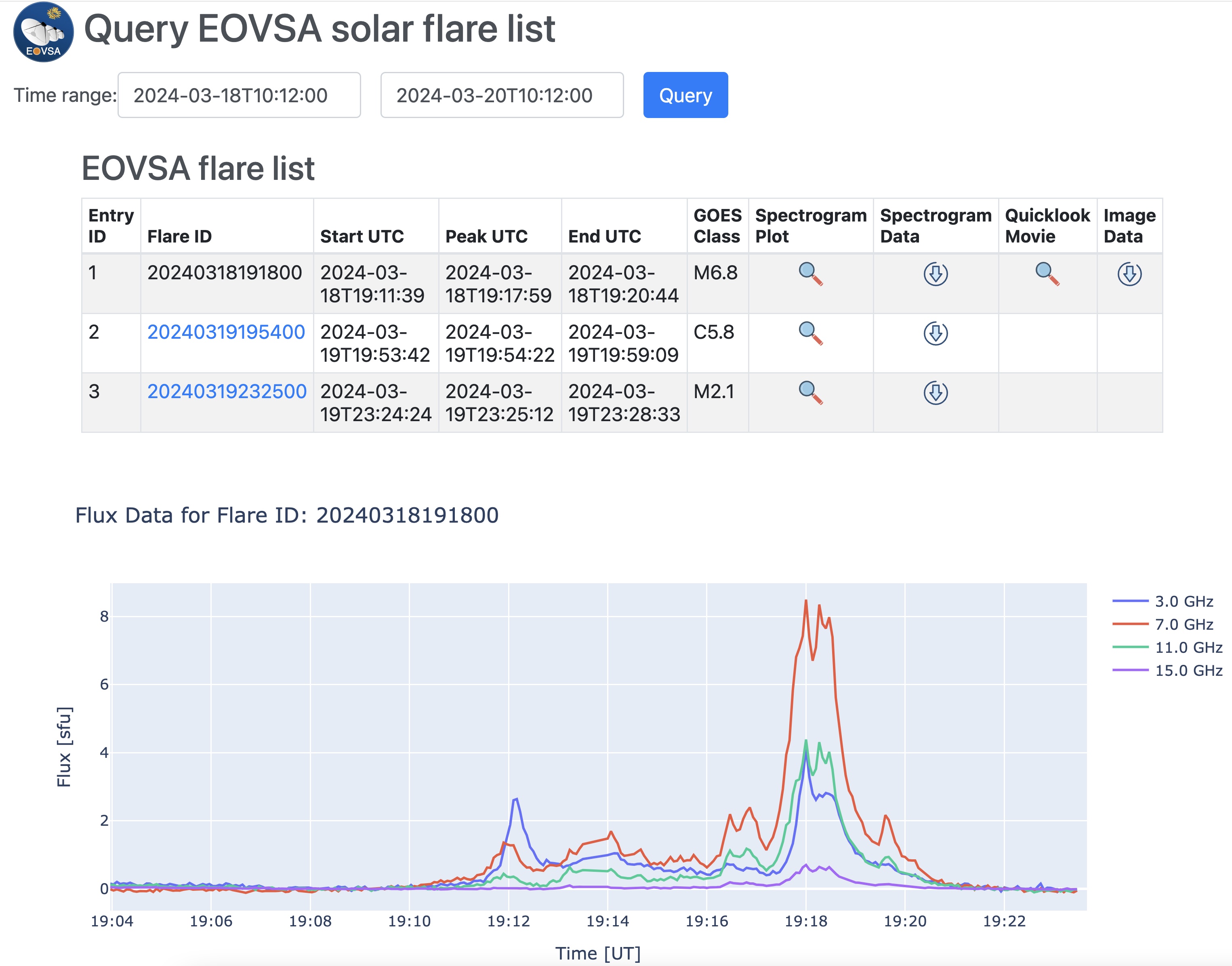
Flare list	The EOVSA event table for the selected date or UTC range, including event timing and links to available quicklook and data products.	Scroll to Events, adjust the UTC range if needed, and select a flare ID or event row.
Flare quicklooks and data	Interactive TP/XP flare spectra plus links to available quicklook plots, movies, images, event spectrogram FITS files, and multi-frequency image products.	Inspect the quicklooks first, then follow the event's data or image links to download the needed files. Availability varies by event.

Quick guide to the EOVSA Data Browser

The Data Browser is primarily the Level 1 discovery and download interface. Raw or calibrated visibility data, reprocessing, and products missing from the site should be requested through the EOVSA data request form.

Data product levels

Level 0: raw visibility data

Full-resolution Interim Database (IDB) visibility data are stored in Miriad format. These products are intended mainly for experienced users who need the original visibility data.

The former NJIT directory listings for IDB and UDB data are not an anonymous download interface. An older public IDB archive remains available from the UC Berkeley EOVSA archive. For recent IDB data, 1-minute-averaged UDB data, or dates not available there, use the EOVSA data request form.

Level 0.5: calibrated visibility data

Calibrated and self-calibrated visibility data are CASA measurement sets. They provide the greatest flexibility for imaging and spatially resolved spectral analysis, but require experience with CASA or sunCASA. See EOVSA_Data_Analysis_Tutorial for the visibility-data workflow.

Some flare records include calibrated or self-calibrated measurement-set archives. Availability is event dependent. If the desired files are not listed for an event, submit a data request rather than constructing a direct directory URL.

Level 1: spectrograms and images in FITS format

Level 1 products are the recommended starting point for most users. They are science-ready FITS products with calibrated physical units:

• Spectrogram intensity is in solar flux units (sfu).
• Image intensity is brightness temperature (K).
• Images use helioprojective, World Coordinate System (WCS)-compatible coordinates and can be read with Astropy, SunPy, or SSWIDL.

Level 1 products are suitable for context studies and many quantitative applications. Use care with spatially resolved spectral analysis, especially when an event product has limited image quality or incomplete frequency coverage.

Synoptic products

• Full-day TP spectrogram: calibrated total flux at full time and frequency resolution. This is the preferred starting point for quantitative spectral measurements.
• Full-day XP spectrogram: cross-power product formed from intermediate baselines. XP suppresses extended background and can reveal temporal structure more clearly, but it can resolve out large sources and therefore underestimate their total flux.
• Daily synoptic images: one representative full-disk image in each of seven EOVSA bands, produced using a long integration for improved uv coverage.
• Synoptic image sequence products: additional full-disk images within an observing day when available. Sequence products are separate from the representative daily products.

Event-based products

• Flare TP and XP spectrograms: event-cropped, full-resolution spectrograms. For events since mid-October 2024, both TP and XP are generally provided. TP should be used for total-flux measurements; XP is useful for emphasizing compact and rapidly varying emission.
• Flare spectral images: multi-frequency image cubes, normally at 12-second cadence and up to ten frequency bands. Products are pipeline calibrated and registered in helioprojective coordinates.

Summary of Level 1 products

EOVSA Level 1 data products and naming patterns

Category	Product	Typical naming pattern	Access
Full-day spectrograms	TP spectrogram	EOVSA_TPall_yyyymmdd.fts	EOVSA Data Browser → select a UTC date → Product Downloads
	XP spectrogram	EOVSA_XPall_yyyymmdd.fts
Synoptic images	Daily product	Current: eovsa.synoptic_daily.yyyymmddTHHMMSSZ.sXX-YY.tb.disk.fits Legacy v1.0: eovsa_yyyymmdd.spwXX-YY.tb.disk.fits
	Sequence product	eovsa.synoptic.yyyymmddTHHMMSSZ.sXX-YY.tb.disk.fits
Flare spectrograms	TP spectrogram	eovsa.spec_tp.flare_id_YYYYMMDDHHMM.fits	EOVSA Data Browser → Events
	XP spectrogram	eovsa.spec_xp.flare_id_YYYYMMDDHHMM.fits
Flare spectral images	Multi-frequency image cube	eovsa.lev1_mbd_12s.YYYY-MM-DDTHHMMSSZ.image.fits

The browser may offer FITS and JP2 representations of a synoptic image. FITS is the science-data format; JP2 is a convenient image representation. Full-day TP/XP spectrograms are FITS-only and are not tied to a synoptic image product version.

Synoptic image bands and product versions

The current browser labels the fourth band as 6.9 GHz. Older documentation and v1.0 filenames may call the same band 6.8 GHz. The spw or s range is a filename identifier; use the frequency metadata in the FITS file for analysis.

Band ID	Browser label	v1.0 spectral-window range	v3.0 spectral-window range
bd01	1.4 GHz	00-01	00-01
bd02	3.0 GHz	02-05	02-04
bd03	4.5 GHz	06-10	05-10
bd04	6.9 GHz	11-20	11-20
bd05	10.2 GHz	21-30	21-30
bd06	13.9 GHz	31-43	31-43
bd07	17.0 GHz	44-49	44-49

EOVSA full-disk synoptic image bands

v1.0 and v3.0 identify different releases of the synoptic imaging products. They are not interchangeable filename aliases. The browser shows the versions available for the selected date and normally defaults to the newest available version. If a selected version has no product for a date or band, choose another listed version or submit a data request; do not silently substitute one version for another in a reproducible analysis.

Browsing and downloading from the EOVSA Data Browser

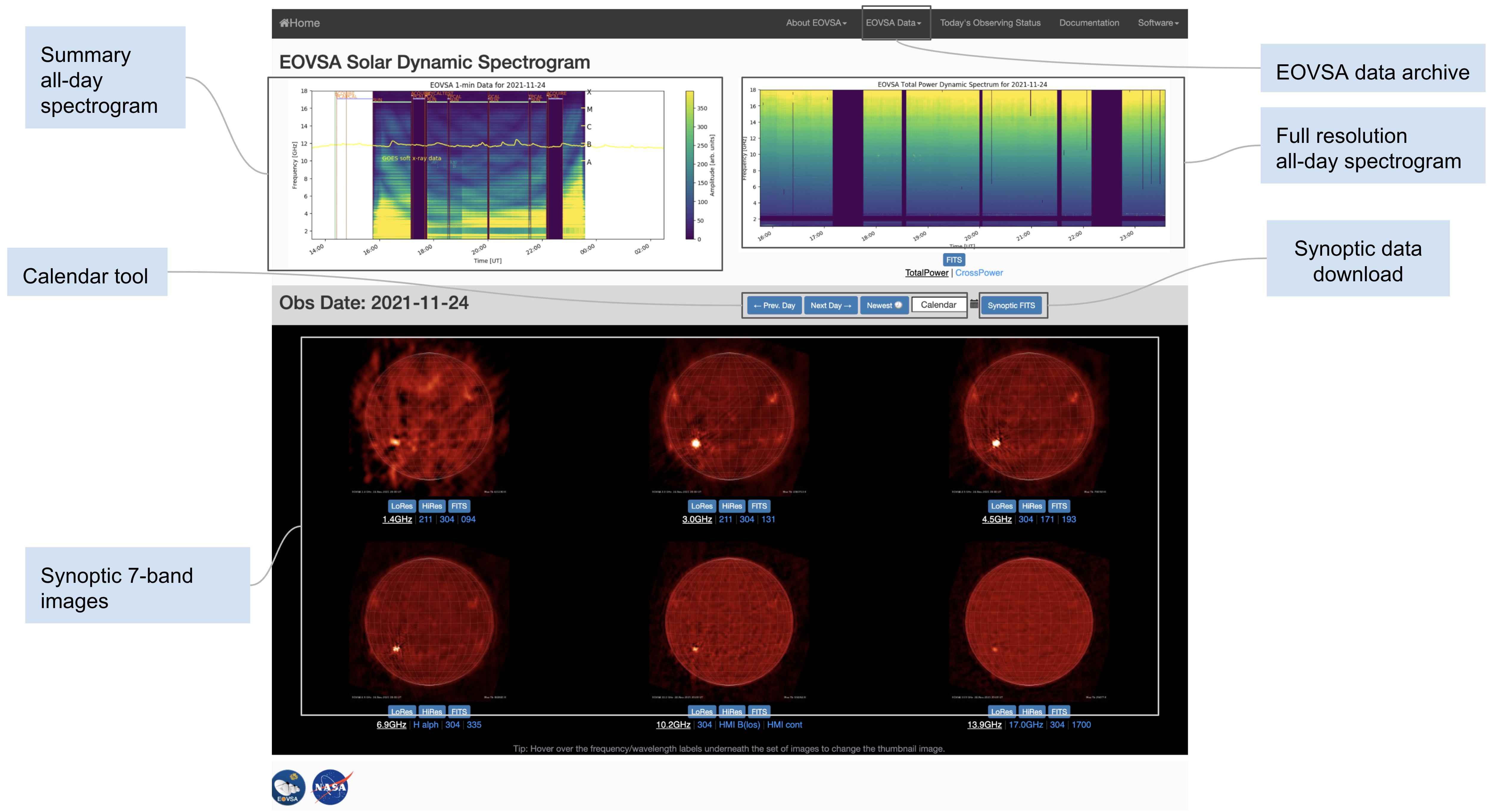
Synoptic data

1. Open the EOVSA Data Browser.
2. Select Tour for a guided walk-through of the main controls, or continue with the steps below.
3. Select the observing date in UTC. The Coverage view indicates whether imaging and/or spectrogram previews are available.
4. Inspect the previews and select the desired Product Version and EOVSA band.
5. Select Sign in for downloads. Register with an email address if needed and follow the access link sent by the site.
6. Select Product Downloads.
7. Download the full-day TP/XP spectrograms and/or the desired daily or sequence synoptic image products. Use the checkboxes to choose product kind and file format.

Product downloads use the signed-in browser session. Anonymous direct FITS URLs and old directory paths can return HTTP 401 or 403 and should not be used as a notebook data-delivery mechanism.

Flare data

1. Open the Events section of the EOVSA Data Browser.
2. Select a UTC date or adjust the event time range.
3. Choose an event and compare its TP and XP quicklook spectrograms.
4. Use the data links to download both TP and XP FITS files when available.
5. If the event has an image-data link, open it and download one or more multi-frequency image cubes. Calibrated and self-calibrated measurement-set archives may also be listed for some events.

Reading and Using Level 1 Data

Introduction

All Level 1 products are FITS files. The spectrogram extensions contain the measurements, frequency axis, and time axis. The images use standard WCS-compatible helioprojective coordinates. The examples below show maintained Python/Colab workflows and the original SSWIDL workflows.

Simple local Python scripts

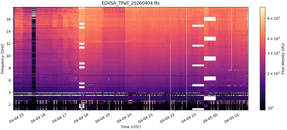
These examples use products from 2026-04-04 and read files that are already on your computer. Put each script in the same directory as the downloaded FITS files, edit the filename variables at the top, and run it locally. No Colab upload and no network access are required.

Both scripts use the same read_eovsa_spectrogram() function. It recognizes the full-day time convention (MJD plus milliseconds) and the flare time convention (Julian Date), as well as the SFREQ and FGHZ frequency columns. The function is repeated so that each script can be copied and run by itself.

Install the required packages once:

python -m pip install numpy matplotlib astropy "sunpy[map]"

Synoptic spectrogram and image

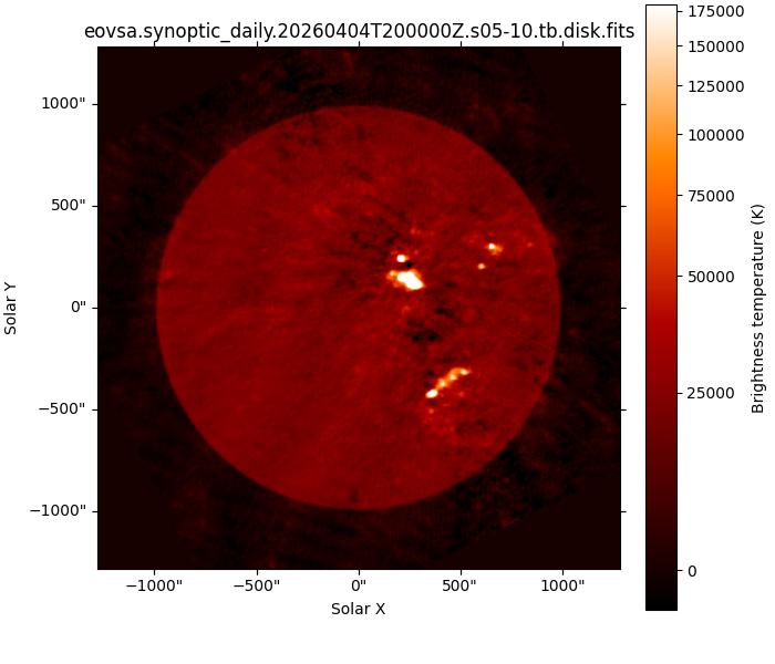
Save the following as plot_eovsa_synoptic.py. Set TP_FILE and IMAGE_FILE to the actual filenames downloaded through Product Downloads, then run python plot_eovsa_synoptic.py. The image uses the same sdoaia304 color map, asinh stretch, and fixed band-dependent temperature scale as the EOVSA Data Browser preview.

from pathlib import Path

import matplotlib.pyplot as plt
import numpy as np
import sunpy.map
from astropy.io import fits
from astropy.time import Time
from astropy.visualization import AsinhStretch, ImageNormalize
from matplotlib.colors import LogNorm

# Change these two filenames.
TP_FILE = Path("EOVSA_TPall_20260404.fts")
IMAGE_FILE = Path("eovsa.synoptic_daily.20260404T200000Z.s05-10.tb.disk.fits")

# Fixed brightness-temperature limits used by the EOVSA Data Browser previews.
SITE_IMAGE_LIMITS = {
    "s00-01": (-18_000, 700_000),
    "s02-04": (-8_000, 300_000),
    "s05-10": (-4_800, 180_000),
    "s11-20": (-3_400, 130_000),
    "s21-30": (-2_100, 80_000),
    "s31-43": (-1_600, 60_000),
    "s44-49": (-1_600, 60_000),
}

def read_eovsa_spectrogram(filename):
    """Read a full-day or flare EOVSA spectrogram FITS file."""
    with fits.open(filename) as hdul:
        data = np.array(hdul[0].data, dtype=float)

        frequency_name = next(
            name for name in hdul[1].columns.names
            if name.lower() in ("sfreq", "fghz")
        )
        frequency_ghz = np.asarray(
            hdul[1].data[frequency_name], dtype=float
        ).squeeze()

        time_table = hdul[2].data
        time_names = {name.lower(): name for name in time_table.names}
        if {"mjd", "time"}.issubset(time_names):
            mjd = np.asarray(time_table[time_names["mjd"]], dtype=float)
            milliseconds = np.asarray(time_table[time_names["time"]], dtype=float)
            times = Time(mjd + milliseconds / 86400000.0, format="mjd")
        elif "time" in time_names:
            times = Time(
                np.asarray(time_table[time_names["time"]], dtype=float),
                format="jd",
            )
        else:
            raise ValueError(f"Unrecognized time columns: {time_table.names}")

    expected_shape = (frequency_ghz.size, len(times))
    if data.shape == expected_shape[::-1]:
        data = data.T
    if data.shape != expected_shape:
        raise ValueError(
            f"Data shape {data.shape} does not match frequency/time axes {expected_shape}"
        )
    return data, frequency_ghz, times.datetime


# Read and plot the full-day total-power spectrogram.
spectrum, frequency_ghz, times = read_eovsa_spectrogram(TP_FILE)

positive = spectrum[np.isfinite(spectrum) & (spectrum > 0)]
vmin, vmax = np.percentile(positive, [5, 99.5])
plot_spectrum = np.ma.masked_less_equal(spectrum, 0)
step = max(1, spectrum.shape[1] // 5000)

fig, ax = plt.subplots(figsize=(11, 5), constrained_layout=True)
image = ax.pcolormesh(
    times[::step], frequency_ghz, plot_spectrum[:, ::step],
    shading="auto", cmap="magma", norm=LogNorm(vmin=vmin, vmax=vmax),
)
ax.set(xlabel="Time (UTC)", ylabel="Frequency (GHz)", title=TP_FILE.name)
fig.colorbar(image, ax=ax, label="Flux density (sfu)")
fig.autofmt_xdate()
plt.show()

# Read and plot one full-disk synoptic image.
with fits.open(IMAGE_FILE) as hdul:
    map_data = np.array(hdul[1].data, dtype=float).squeeze()
    map_header = hdul[1].header.copy()

band_tag = next((tag for tag in SITE_IMAGE_LIMITS if tag in IMAGE_FILE.name), None)
if band_tag is None:
    raise ValueError("Cannot match the image filename to a standard EOVSA band")

vmin, vmax = SITE_IMAGE_LIMITS[band_tag]
eovsa_map = sunpy.map.Map(map_data, map_header)
cmap = plt.get_cmap("sdoaia304").copy()
cmap.set_bad("black")
norm = ImageNormalize(vmin=vmin, vmax=vmax, stretch=AsinhStretch(a=0.15))

fig = plt.figure(figsize=(7, 6), constrained_layout=True)
ax = fig.add_subplot(projection=eovsa_map)
image = eovsa_map.plot(axes=ax, cmap=cmap, norm=norm)
ax.set(xlabel="Solar X", ylabel="Solar Y", title=IMAGE_FILE.name)
ax.grid(False)
fig.colorbar(image, ax=ax, label="Brightness temperature (K)")
plt.show()

Full-day EOVSA total-power spectrogram for 2026-04-04, produced by the Python script.

EOVSA s05-10 synoptic image (about 4.5 GHz) for 2026-04-04, produced by the Python script.

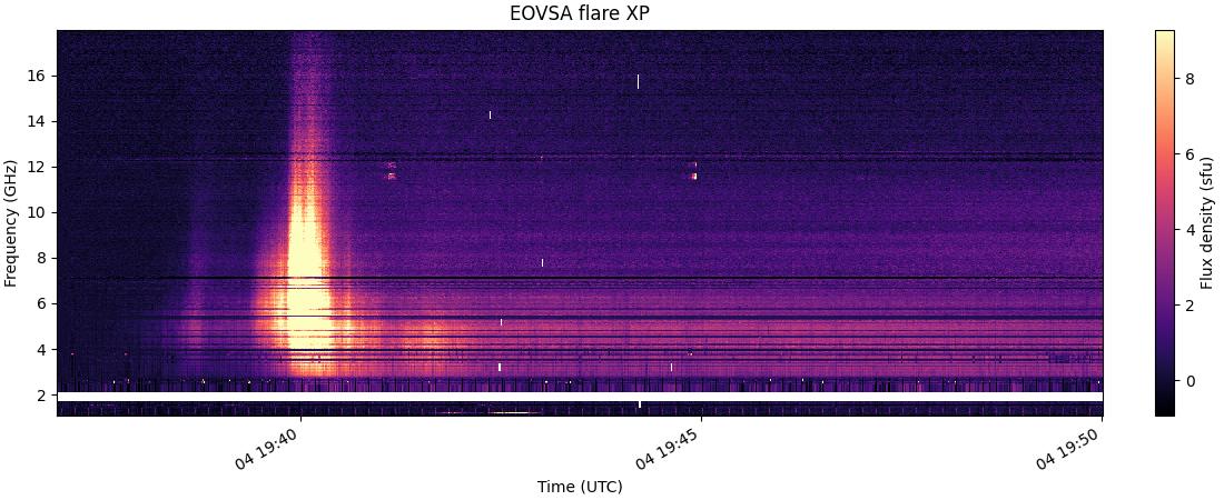
Flare XP spectrogram and EOVSA-on-AIA image

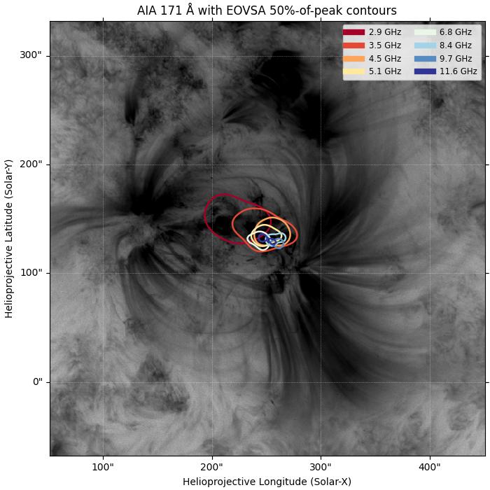
Save the following as plot_eovsa_flare.py. Change the three filenames to files from one event and run python plot_eovsa_flare.py. This example uses the 2026-04-04 19:39 UT flare. AIA_FILE should be an AIA 171 Å FITS image close to the EOVSA image time. The final plot uses AIA as the background and overlays the eight quicklook frequencies shown for this event.

from pathlib import Path

import astropy.units as u
import matplotlib.pyplot as plt
import numpy as np
import sunpy.map
from astropy.coordinates import SkyCoord
from astropy.io import fits
from astropy.time import Time
from matplotlib.lines import Line2D

# Change these three filenames.
XP_FILE = Path("eovsa.spec_xp.flare_id_202604041939.fits")
IMAGE_FILE = Path("eovsa.lev1_mbd_12s.2026-04-04T193957Z.image.fits")
AIA_FILE = Path("aia.lev1_euv_12s.2026-04-04T194403Z.171.image.fits")
ZOOM_ARCSEC = 200

def read_eovsa_spectrogram(filename):
    """Read a full-day or flare EOVSA spectrogram FITS file."""
    with fits.open(filename) as hdul:
        data = np.array(hdul[0].data, dtype=float)

        frequency_name = next(
            name for name in hdul[1].columns.names
            if name.lower() in ("sfreq", "fghz")
        )
        frequency_ghz = np.asarray(
            hdul[1].data[frequency_name], dtype=float
        ).squeeze()

        time_table = hdul[2].data
        time_names = {name.lower(): name for name in time_table.names}
        if {"mjd", "time"}.issubset(time_names):
            mjd = np.asarray(time_table[time_names["mjd"]], dtype=float)
            milliseconds = np.asarray(time_table[time_names["time"]], dtype=float)
            times = Time(mjd + milliseconds / 86400000.0, format="mjd")
        elif "time" in time_names:
            times = Time(
                np.asarray(time_table[time_names["time"]], dtype=float),
                format="jd",
            )
        else:
            raise ValueError(f"Unrecognized time columns: {time_table.names}")

    expected_shape = (frequency_ghz.size, len(times))
    if data.shape == expected_shape[::-1]:
        data = data.T
    if data.shape != expected_shape:
        raise ValueError(
            f"Data shape {data.shape} does not match frequency/time axes {expected_shape}"
        )
    return data, frequency_ghz, times.datetime


xp, xp_frequency, xp_times = read_eovsa_spectrogram(XP_FILE)

finite = xp[np.isfinite(xp)]
vmin, vmax = np.percentile(finite, [1, 99.0])

fig, ax = plt.subplots(figsize=(11, 4.5), constrained_layout=True)
image = ax.pcolormesh(
    xp_times, xp_frequency, xp,
    shading="auto", cmap="magma", vmin=vmin, vmax=vmax,
)
ax.set(xlabel="Time (UTC)", ylabel="Frequency (GHz)", title="EOVSA flare XP")
fig.colorbar(image, ax=ax, label="Flux density (sfu)")
fig.autofmt_xdate()
plt.show()

# Overlay the eight quicklook frequencies on the AIA 171 Å image.
with fits.open(IMAGE_FILE) as hdul:
    cube = np.array(hdul[1].data, dtype=float)
    image_header = hdul[1].header.copy()
    cube_frequency_hz = np.asarray(hdul[2].data["cfreqs"], dtype=float)

cube_frequency_ghz = cube_frequency_hz / 1e9
colors = plt.get_cmap("RdYlBu")(np.linspace(0, 1, cube_frequency_ghz.size)
)


aia_map = sunpy.map.Map(AIA_FILE)
fig = plt.figure(figsize=(7, 7), constrained_layout=True)
ax = fig.add_subplot(projection=aia_map)
aia_map.plot(axes=ax, cmap="gray_r", clip_interval=(1, 99.8) * u.percent)

legend_items = []
for plane, color in enumerate(colors):
    header = image_header.copy()
    header["RESTFRQ"] = float(cube_frequency_hz[plane])
    eovsa_map = sunpy.map.Map(cube[plane], header)
    eovsa_map.draw_contours(
        levels=[50] * u.percent,
        axes=ax, colors=[color], linewidths=1.8,
    )
    legend_items.append(
        Line2D([], [], color=color, linewidth=6,
               label=f"{cube_frequency_ghz[plane]:.1f} GHz")
    )

# Center the view on the EOVSA image; change ZOOM_ARCSEC if desired.
corners = SkyCoord(
    Tx=(image_header["CRVAL1"] + np.array([-ZOOM_ARCSEC, ZOOM_ARCSEC])) * u.arcsec,
    Ty=(image_header["CRVAL2"] + np.array([-ZOOM_ARCSEC, ZOOM_ARCSEC])) * u.arcsec,
    frame=aia_map.coordinate_frame,
)
x_pixels, y_pixels = aia_map.world_to_pixel(corners)
ax.set_xlim(np.clip(x_pixels.value, 0, aia_map.data.shape[1] - 1))
ax.set_ylim(np.clip(y_pixels.value, 0, aia_map.data.shape[0] - 1))
ax.legend(handles=legend_items, loc="upper right", ncols=2, fontsize="small")
ax.set_title("AIA 171 Å with EOVSA 50%-of-peak contours")
plt.show()

EOVSA XP spectrogram for the 2026-04-04 19:39 UT flare.

AIA 171 Å image with eight EOVSA frequency contours for the 2026-04-04 flare.

Optional Colab tutorials

The local scripts above are the shortest route for files already downloaded to a computer. The longer Colab notebooks provide guided explanations, additional checks, and optional exercises:

• Basic 1: read and plot EOVSA synoptic FITS products
• Basic 2: compare EOVSA flare TP/XP spectrograms and plot an image cube

Colab cannot use the EOVSA site's signed-in browser session. If using a Colab notebook, download the requested products through the EOVSA Data Browser and upload them when prompted.

Troubleshooting

• File not found: put the script in the same directory as the downloaded files or enter the full local path in the filename variables.
• Missing Python package: run python -m pip install numpy matplotlib astropy "sunpy[map]" in the same Python environment used to run the script.
• HTTP 401 or 403 while obtaining data: return to the EOVSA Data Browser, sign in, and download through Product Downloads or the event's data links. Do not retry an old direct directory URL.
• No products for a version: check the selected UTC date and choose a product version explicitly listed by the browser.
• Unexpected spectrogram range: adjust the spectrogram percentile values and document the limits used for science analysis. The synoptic image limits are intentionally fixed by band to match the EOVSA Data Browser previews.

SSWIDL tutorials

The following examples are retained for SSWIDL users. Download the files through the EOVSA Data Browser first and use the downloaded filename in the examples.

Synoptic spectrograms

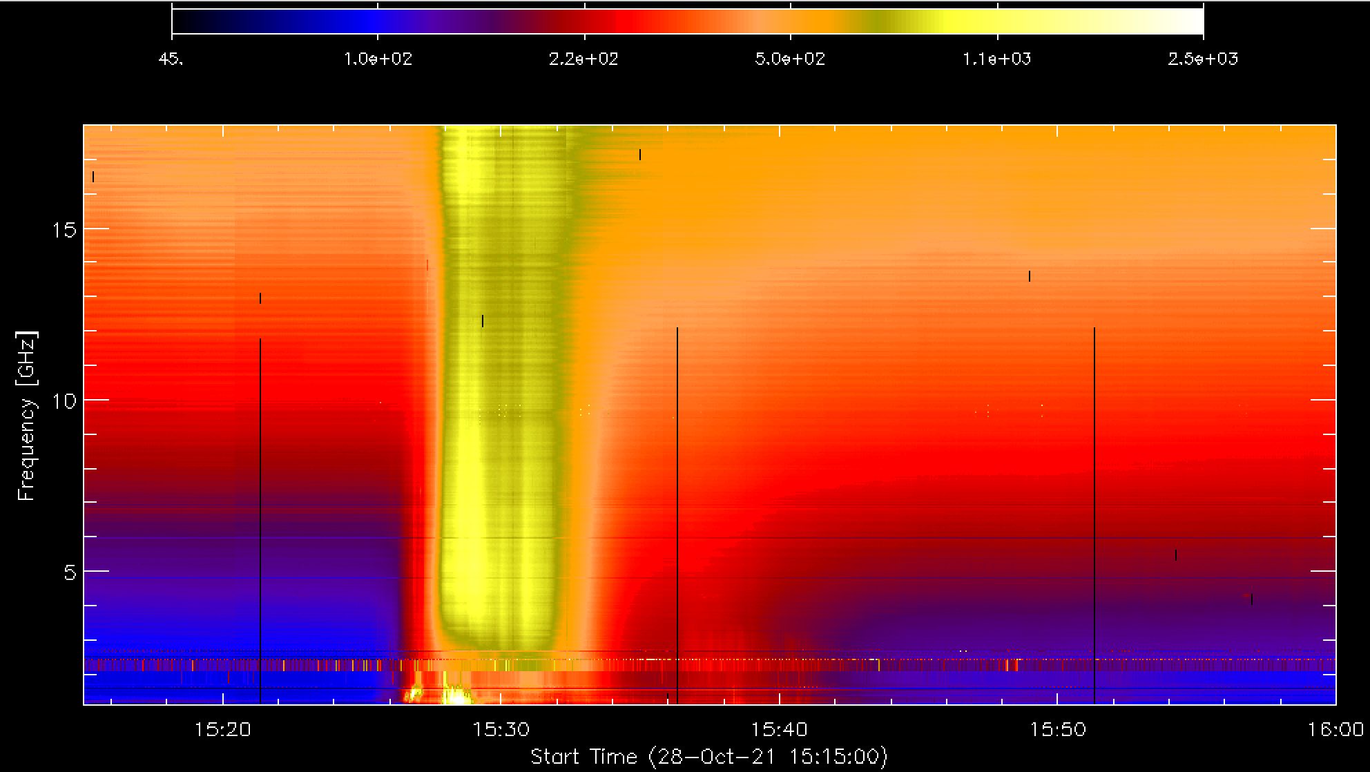
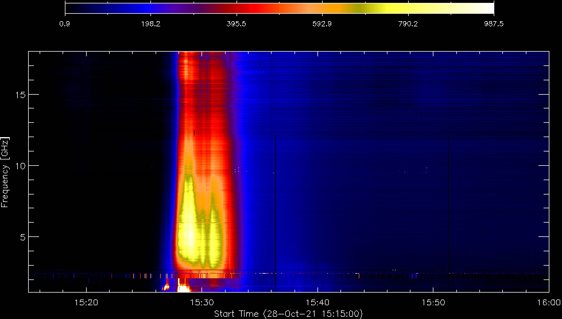
This example uses SSWIDL's mrdfits to read a full-day total-power FITS file and the spectrogram object to display it. The example date is the 2021 October 28 X1 flare; its products can be found by selecting 2021-10-28 in the EOVSA Data Browser.

; Read the FITS file using mrdfits
filename = 'EOVSA_TPall_20211028.fts'
spec = mrdfits(filename,0) ; Array of amplitudes in sfu: [ntime, nfreq]
freq = mrdfits(filename,1) ; Frequency-information structure: [nfreq]
time = mrdfits(filename,2) ; UT time information: [ntime]
fghz = freq.sfreq          ; Center frequencies in GHz
timeut = anytim(time)      ; Convert the time into SSWIDL anytim format

ntime = n_elements(timeut)
nfreq = n_elements(fghz)

; Convert the information into a spectrogram object
s = spectrogram(spec, timeut, fghz)

; Make a simple plot
window,/free,xsiz=1024,ysiz=600
; Find limits from the 5th to 95th percentiles to reduce outlier influence
sarr = sort(spec)
dlim = minmax(spec[sarr[n_elements(sarr)*0.05:n_elements(sarr)*0.95]])
; Add display margins below and above the percentile range
s.set,drange=dlim*[0.5,5]
loadct,5
s.plot,/log,timerange=['2021-10-28T15:15:00','2021-10-28T16:00:00'],/xsty,/ysty,ytitle='Frequency [GHz]',charsize=1.5

The following optional example subtracts the mean spectrum from a selected pre-flare interval. Keep the original spec array unchanged and store the result in spec_sub.

; Select a pre-flare background interval
timebkg = ['2021-10-28T15:15', '2021-10-28T15:20']
dt0 = min(abs(timeut - anytim(timebkg[0])), bkg_i0)
dt1 = min(abs(timeut - anytim(timebkg[1])), bkg_i1)
spec_bkg = mean(spec[bkg_i0:bkg_i1,*], dimension=1)
spec_sub = spec - rebin(reform(spec_bkg, 1, nfreq), ntime, nfreq)

; Create and plot the background-subtracted spectrogram
s = spectrogram(spec_sub, timeut, fghz)
window,/free,xsiz=1024,ysiz=600
s->set,drange=dlim*[0.01,2]
loadct,5
s.plot,/linear,timerange=['2021-10-28T15:15:00','2021-10-28T16:00:00'],/xsty,/ysty,ytitle='Frequency [GHz]',charsize=1.5

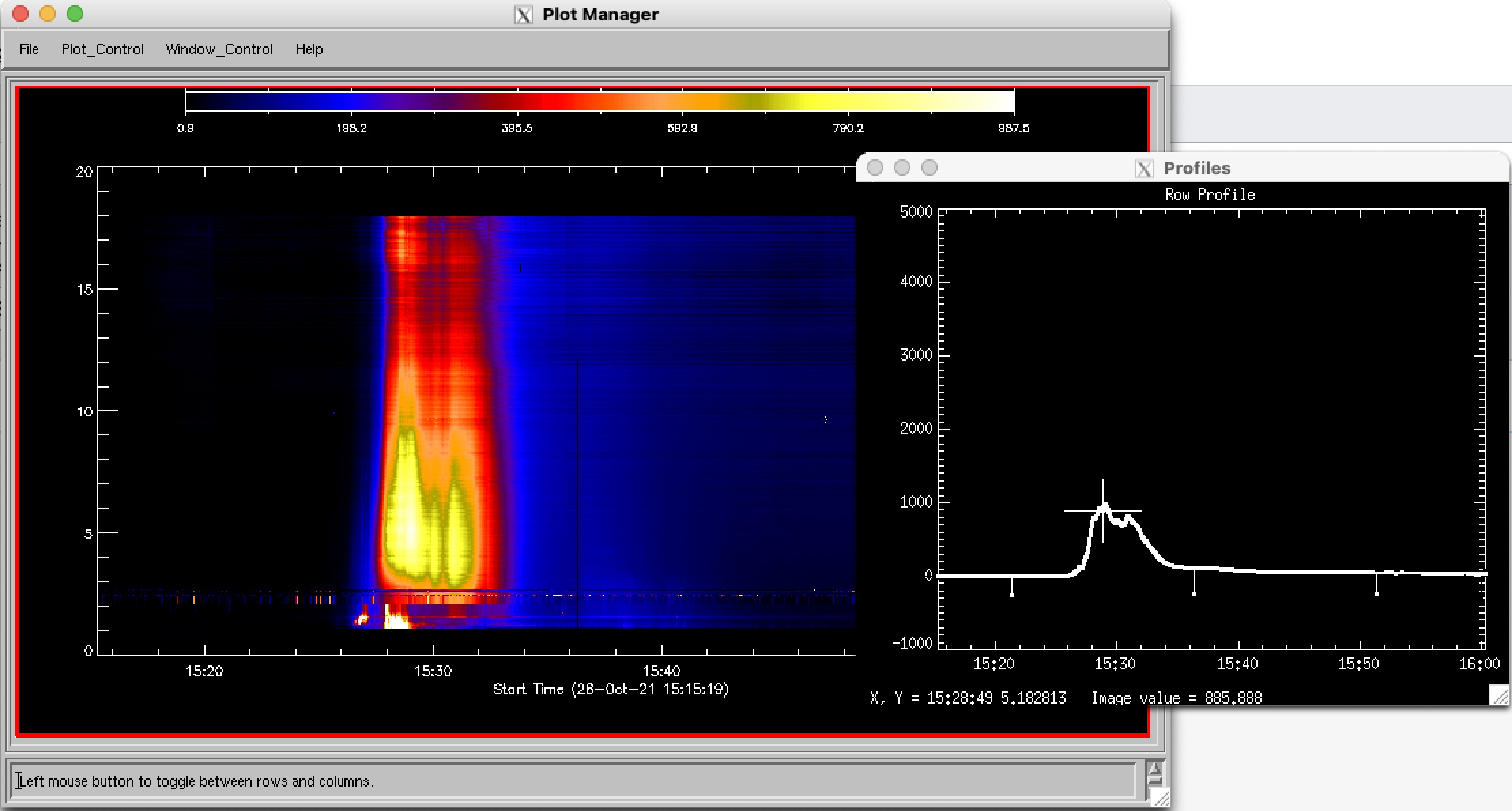
The spectrogram object can also be opened in plotman. To examine light curves, select plot_Control → Image or Spectrogram Profiles → Rows or Columns.

s->set,timerange=['2021-10-28T15:15:00','2021-10-28T16:00:00']
s->plotman

Synoptic images

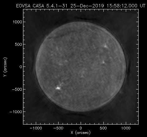
Read a synoptic image with read_sdo, convert it to a map with index2map, and display it with plot_map. The filename below is a legacy v1.0 example; substitute the actual filename downloaded from the browser when using another date or product version.

read_sdo,'eovsa_20191225.spw11-20.tb.disk.fits',header,data,/UNCOMP_DELETE
index2map,header,data,eomap
plot_map,eomap

Event-based spectrograms

For event-based products, the time table contains Julian Date (JD) values rather than the full-day product's time convention. The following function converts JD to SSWIDL anytim seconds. Most event spectrogram products have already had a pre-flare background removed, so inspect the product before applying another background subtraction.

; Convert Julian Date to SSWIDL anytim seconds since 1979-01-01 00:00:00 UTC
function jd2anytim, jd
  jd0 = 2443874.5
  sec_per_day = 86400.0
  return, (jd - jd0) * sec_per_day
end

; Read an event-based FITS file
filename = 'eovsa.spec.flare_id_20211028152600.fits'
spec = mrdfits(filename, 0)      ; [ntime, nfreq] amplitudes in sfu
freq = mrdfits(filename, 1)      ; Frequency-information structure: [nfreq]
time = mrdfits(filename, 2)      ; Structure with a JD field named time: [ntime]

fghz = freq.fghz                 ; Center frequencies in GHz
timeut = jd2anytim(time.time)    ; Convert JD to SSWIDL anytim seconds

; Continue with the spectrogram creation and plotting commands above

Tip: After timeut = jd2anytim(time.time), continue with the synoptic example's spectrogram, plotting, and plotman commands. Newer event files distinguish TP and XP in names such as eovsa.spec_tp.flare_id_YYYYMMDDHHMM.fits and eovsa.spec_xp.flare_id_YYYYMMDDHHMM.fits.

Citation, acknowledgment, and data use

Before publication, review the current OVSA Data Policy. It contains the authoritative acknowledgment, citation, contact, and authorship guidance.

For work using EOVSA data, the current acknowledgment can be adapted from:

EOVSA was designed, built, and is now operated by the New Jersey Institute of Technology (NJIT) as a community facility. EOVSA solar operations are supported by NSF grant AGS-2436999 to NJIT.

Papers using EOVSA data should cite Gary et al. (2018), Microwave and Hard X-Ray Observations of the 2017 September 10 Solar Limb Flare, ApJ 863, 83 (DOI). See the data policy for current co-authorship and Scientist-on-Duty guidance.

The EOVSA citation landing page describes the maintained Level 1 collection. Its collection DOI is currently pending; do not cite a DOI as assigned until that page provides one.

Requesting EOVSA data or analysis assistance

The public product list is not complete for every date or every processing level. Submit the EOVSA data request form if:

• a desired date or event is missing;
• raw, calibrated, or self-calibrated visibility data are required;
• higher time/frequency resolution or reprocessing is needed; or
• interpretation requires help from an EOVSA team member.

The team normally responds within 2--3 working days. Contacting the team early is recommended because product limitations and instrumental effects may not be evident from the files alone. Follow the OVSA Data Policy for acknowledgment and authorship requirements.

Migrated from MediaWiki page EOVSA Data Products, latest revision 16302 (2026-08-14T02:28:36Z).